2.4: Solution Sets
- Page ID
- 70189

\( \newcommand{\vecs}[1]{\overset { \scriptstyle \rightharpoonup} {\mathbf{#1}} } \)
\( \newcommand{\vecd}[1]{\overset{-\!-\!\rightharpoonup}{\vphantom{a}\smash {#1}}} \)
\( \newcommand{\dsum}{\displaystyle\sum\limits} \)
\( \newcommand{\dint}{\displaystyle\int\limits} \)
\( \newcommand{\dlim}{\displaystyle\lim\limits} \)
\( \newcommand{\id}{\mathrm{id}}\) \( \newcommand{\Span}{\mathrm{span}}\)
( \newcommand{\kernel}{\mathrm{null}\,}\) \( \newcommand{\range}{\mathrm{range}\,}\)
\( \newcommand{\RealPart}{\mathrm{Re}}\) \( \newcommand{\ImaginaryPart}{\mathrm{Im}}\)
\( \newcommand{\Argument}{\mathrm{Arg}}\) \( \newcommand{\norm}[1]{\| #1 \|}\)
\( \newcommand{\inner}[2]{\langle #1, #2 \rangle}\)
\( \newcommand{\Span}{\mathrm{span}}\)
\( \newcommand{\id}{\mathrm{id}}\)
\( \newcommand{\Span}{\mathrm{span}}\)
\( \newcommand{\kernel}{\mathrm{null}\,}\)
\( \newcommand{\range}{\mathrm{range}\,}\)
\( \newcommand{\RealPart}{\mathrm{Re}}\)
\( \newcommand{\ImaginaryPart}{\mathrm{Im}}\)
\( \newcommand{\Argument}{\mathrm{Arg}}\)
\( \newcommand{\norm}[1]{\| #1 \|}\)
\( \newcommand{\inner}[2]{\langle #1, #2 \rangle}\)
\( \newcommand{\Span}{\mathrm{span}}\) \( \newcommand{\AA}{\unicode[.8,0]{x212B}}\)
\( \newcommand{\vectorA}[1]{\vec{#1}} % arrow\)
\( \newcommand{\vectorAt}[1]{\vec{\text{#1}}} % arrow\)
\( \newcommand{\vectorB}[1]{\overset { \scriptstyle \rightharpoonup} {\mathbf{#1}} } \)
\( \newcommand{\vectorC}[1]{\textbf{#1}} \)
\( \newcommand{\vectorD}[1]{\overrightarrow{#1}} \)
\( \newcommand{\vectorDt}[1]{\overrightarrow{\text{#1}}} \)
\( \newcommand{\vectE}[1]{\overset{-\!-\!\rightharpoonup}{\vphantom{a}\smash{\mathbf {#1}}}} \)
\( \newcommand{\vecs}[1]{\overset { \scriptstyle \rightharpoonup} {\mathbf{#1}} } \)
\(\newcommand{\longvect}{\overrightarrow}\)
\( \newcommand{\vecd}[1]{\overset{-\!-\!\rightharpoonup}{\vphantom{a}\smash {#1}}} \)
\(\newcommand{\avec}{\mathbf a}\) \(\newcommand{\bvec}{\mathbf b}\) \(\newcommand{\cvec}{\mathbf c}\) \(\newcommand{\dvec}{\mathbf d}\) \(\newcommand{\dtil}{\widetilde{\mathbf d}}\) \(\newcommand{\evec}{\mathbf e}\) \(\newcommand{\fvec}{\mathbf f}\) \(\newcommand{\nvec}{\mathbf n}\) \(\newcommand{\pvec}{\mathbf p}\) \(\newcommand{\qvec}{\mathbf q}\) \(\newcommand{\svec}{\mathbf s}\) \(\newcommand{\tvec}{\mathbf t}\) \(\newcommand{\uvec}{\mathbf u}\) \(\newcommand{\vvec}{\mathbf v}\) \(\newcommand{\wvec}{\mathbf w}\) \(\newcommand{\xvec}{\mathbf x}\) \(\newcommand{\yvec}{\mathbf y}\) \(\newcommand{\zvec}{\mathbf z}\) \(\newcommand{\rvec}{\mathbf r}\) \(\newcommand{\mvec}{\mathbf m}\) \(\newcommand{\zerovec}{\mathbf 0}\) \(\newcommand{\onevec}{\mathbf 1}\) \(\newcommand{\real}{\mathbb R}\) \(\newcommand{\twovec}[2]{\left[\begin{array}{r}#1 \\ #2 \end{array}\right]}\) \(\newcommand{\ctwovec}[2]{\left[\begin{array}{c}#1 \\ #2 \end{array}\right]}\) \(\newcommand{\threevec}[3]{\left[\begin{array}{r}#1 \\ #2 \\ #3 \end{array}\right]}\) \(\newcommand{\cthreevec}[3]{\left[\begin{array}{c}#1 \\ #2 \\ #3 \end{array}\right]}\) \(\newcommand{\fourvec}[4]{\left[\begin{array}{r}#1 \\ #2 \\ #3 \\ #4 \end{array}\right]}\) \(\newcommand{\cfourvec}[4]{\left[\begin{array}{c}#1 \\ #2 \\ #3 \\ #4 \end{array}\right]}\) \(\newcommand{\fivevec}[5]{\left[\begin{array}{r}#1 \\ #2 \\ #3 \\ #4 \\ #5 \\ \end{array}\right]}\) \(\newcommand{\cfivevec}[5]{\left[\begin{array}{c}#1 \\ #2 \\ #3 \\ #4 \\ #5 \\ \end{array}\right]}\) \(\newcommand{\mattwo}[4]{\left[\begin{array}{rr}#1 \amp #2 \\ #3 \amp #4 \\ \end{array}\right]}\) \(\newcommand{\laspan}[1]{\text{Span}\{#1\}}\) \(\newcommand{\bcal}{\cal B}\) \(\newcommand{\ccal}{\cal C}\) \(\newcommand{\scal}{\cal S}\) \(\newcommand{\wcal}{\cal W}\) \(\newcommand{\ecal}{\cal E}\) \(\newcommand{\coords}[2]{\left\{#1\right\}_{#2}}\) \(\newcommand{\gray}[1]{\color{gray}{#1}}\) \(\newcommand{\lgray}[1]{\color{lightgray}{#1}}\) \(\newcommand{\rank}{\operatorname{rank}}\) \(\newcommand{\row}{\text{Row}}\) \(\newcommand{\col}{\text{Col}}\) \(\renewcommand{\row}{\text{Row}}\) \(\newcommand{\nul}{\text{Nul}}\) \(\newcommand{\var}{\text{Var}}\) \(\newcommand{\corr}{\text{corr}}\) \(\newcommand{\len}[1]{\left|#1\right|}\) \(\newcommand{\bbar}{\overline{\bvec}}\) \(\newcommand{\bhat}{\widehat{\bvec}}\) \(\newcommand{\bperp}{\bvec^\perp}\) \(\newcommand{\xhat}{\widehat{\xvec}}\) \(\newcommand{\vhat}{\widehat{\vvec}}\) \(\newcommand{\uhat}{\widehat{\uvec}}\) \(\newcommand{\what}{\widehat{\wvec}}\) \(\newcommand{\Sighat}{\widehat{\Sigma}}\) \(\newcommand{\lt}{<}\) \(\newcommand{\gt}{>}\) \(\newcommand{\amp}{&}\) \(\definecolor{fillinmathshade}{gray}{0.9}\)- Understand the relationship between the solution set of \(Ax=0\) and the solution set of \(Ax=b\).
- Understand the difference between the solution set and the column span.
- Recipes: parametric vector form, write the solution set of a homogeneous system as a span.
- Pictures: solution set of a homogeneous system, solution set of an inhomogeneous system, the relationship between the two.
- Vocabulary words: homogeneous/inhomogeneous, trivial solution.
In this section we will study the geometry of the solution set of any matrix equation \(Ax=b\).
Homogeneous Systems
The equation \(Ax=b\) is easier to solve when \(b=0\text{,}\) so we start with this case.
A system of linear equations of the form \(Ax=0\) is called homogeneous.
A system of linear equations of the form \(Ax=b\) for \(b\neq 0\) is called inhomogeneous.
A homogeneous system is just a system of linear equations where all constants on the right side of the equals sign are zero.
A homogeneous system always has the solution \(x=0\). This is called the trivial solution. Any nonzero solution is called nontrivial.
The equation \(Ax=0\) has a nontrivial solution \(\iff\) there is a free variable \(\iff\) \(A\) has a column without a pivot position.
What is the solution set of \(Ax=0\text{,}\) where
\[A=\left(\begin{array}{ccc}1&3&4\\2&-1&2\\1&0&1\end{array}\right)?\nonumber\]
Solution
We form an augmented matrix and row reduce:
\[\left(\begin{array}{ccc|c}1&3&4&0\\2&-1&2&0\\1&0&1&0\end{array}\right) \quad\xrightarrow{\text{RREF}}\quad \left(\begin{array}{ccc|c}1&0&0&0\\0&1&0&0\\0&0&1&0\end{array}\right).\nonumber\]
The only solution is the trivial solution \(x=0\).
When we row reduce the augmented matrix for a homogeneous system of linear equations, the last column will be zero throughout the row reduction process. We saw this in the last Example \(\PageIndex{1}\):
\[\left(\begin{array}{ccc|c}1&3&4&0\\2&-1&2&0\\1&0&1&0\end{array}\right)\nonumber\]
So it is not really necessary to write augmented matrices when solving homogeneous systems.
When the homogeneous equation \(Ax=0\) does have nontrivial solutions, it turns out that the solution set can be conveniently expressed as a span.
Consider the following matrix in reduced row echelon form:
\[A=\left(\begin{array}{cccc}1&0&-8&-7 \\ 0&1&4&3 \\ 0&0&0&0\end{array}\right).\nonumber\]
The matrix equation \(Ax=0\) corresponds to the system of equations
\[\left\{\begin{array}{rrrrrrrrl} x_1&{}&{}& -& 8x_3 &-& 7x_4 &=& 0 \\ {}&{}& x_2 &+& 4x_3 &+& 3x_4 &=& 0.\end{array}\right.\nonumber\]
We can write the parametric form as follows:
\[\left\{\begin{array}{rrrrc} x_1 &=& 8x_3 &+& 7x_4 \\ x_2 &=& -4x_3 &-& 3x_4 \\ x_3 &=& x_3 &{}&{} \\ x_4 &=& {}&{}& x_4.\end{array}\right.\nonumber\]
We wrote the redundant equations \(x_3=x_3\) and \(x_4=x_4\) in order to turn the above system into a vector equation:
\[x=\left(\begin{array}{c}x_1 \\ x_2 \\ x_3 \\ x_4\end{array}\right)=x_3 \left(\begin{array}{c}8\\-4\\1\\0\end{array}\right)+x_4 \left(\begin{array}{c}7\\-3\\0\\1\end{array}\right).\nonumber\]
This vector equation is called the parametric vector form of the solution set. Since \(x_3\) and \(x_4\) are allowed to be anything, this says that the solution set is the set of all linear combinations of \(\left(\begin{array}{c}8\\-4\\1\\0\end{array}\right)\) and \(\left(\begin{array}{c}7\\-3\\0\\1\end{array}\right)\). In other words, the solution set is
\[\text{Span}\left\{\left(\begin{array}{c}8\\-4\\1\\0\end{array}\right),\:\left(\begin{array}{c}7\\-3\\0\\1\end{array}\right)\right\}.\nonumber\]
Here is the general procedure.
Let \(A\) be an \(m\times n\) matrix. Suppose that the free variables in the homogeneous equation \(Ax=0\) are, for example, \(x_3\text{,}\) \(x_6\text{,}\) and \(x_8\).
- Find the reduced row echelon form of \(A\).
- Write the parametric form of the solution set, including the redundant equations \(x_3=x_3\text{,}\) \(x_6=x_6\text{,}\) \(x_8=x_8\). Put equations for all of the \(x_i\) in order.
- Make a single vector equation from these equations by making the coefficients of \(x_3,x_6,\) and \(x_8\) into vectors \(v_3,v_6,\) and \(v_8\text{,}\) respectively.
The solutions to \(Ax=0\) will then be expressed in the form
\[ x = x_3v_3 + x_6v_6 + x_8v_8 \nonumber \]
for some vectors \(v_3,v_6,v_8\) in \(\mathbb{R}^n\text{,}\) and any scalars \(x_3,x_6,x_8\). This is called the parametric vector form of the solution.
In this case, the solution set can be written as \(\text{Span}\{v_3,\,v_6,\,v_8\}.\)
We emphasize the following fact in particular.
The set of solutions to a homogeneous equation \(Ax=0\) is a span.
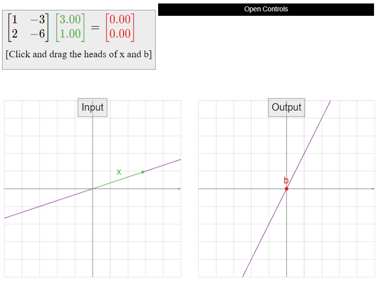
Compute the parametric vector form of the solution set of \(Ax=0\text{,}\) where
\[A=\left(\begin{array}{cc}1&-3\\2&-6\end{array}\right).\nonumber\]
Solution
We row reduce (without augmenting, as suggested in the above Observation \(\PageIndex{2}\)):
\[\left(\begin{array}{cc}1&-3\\2&-6\end{array}\right)\quad\xrightarrow{\text{RREF}}\quad \left(\begin{array}{cc}1&-3\\0&0\end{array}\right).\nonumber\]
This corresponds to the single equation \(x_1 - 3x_2=0\). We write the parametric form including the redundant equation \(x_2=x_2\text{:}\)
\[\left\{\begin{array}{rrc} x_1 &=& 3x_2 \\ x_2 &=& x_2.\end{array}\right.\nonumber\]
We turn these into a single vector equation:
\[x=\left(\begin{array}{c}x_1 \\ x_2\end{array}\right)=x_2\left(\begin{array}{c}3\\1\end{array}\right).\nonumber\]
This is the parametric vector form of the solution set. Since \(x_2\) is allowed to be anything, this says that the solution set is the set of all scalar multiples of \({3\choose 1}\text{,}\) otherwise known as
\[\text{Span}\left\{\left(\begin{array}{c}3\\1\end{array}\right)\right\}.\nonumber\]
We know how to draw the picture of a span of a vector: it is a line. Therefore, this is a picture of the the solution set:
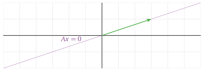
Figure \(\PageIndex{1}\)
Since there were two variables in the above Example \(\PageIndex{3}\), the solution set is a subset of \(\mathbb{R}^2\). Since one of the variables was free, the solution set is a line:
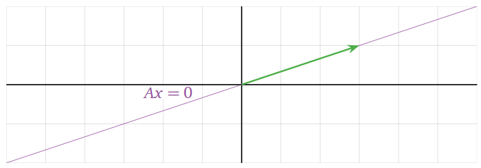
Figure \(\PageIndex{3}\)
In order to actually find a nontrivial solution to \(Ax=0\) in the above Example \(\PageIndex{3}\), it suffices to substitute any nonzero value for the free variable \(x_2\). For instance, taking \(x_2=1\) gives the nontrivial solution \(x = 1\cdot{3\choose 1} = {3\choose 1}.\) Compare to this note in Section 1.3, Note 1.3.1.
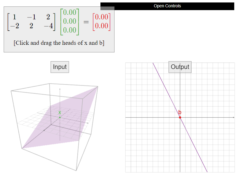
Compute the parametric vector form of the solution set of \(Ax=0\text{,}\) where
\[A=\left(\begin{array}{ccc}1&-1&2\\-2&2&-4\end{array}\right).\nonumber\]
Solution
We row reduce (without augmenting, as suggested in the above Observation \(\PageIndex{2}\)):
\[\left(\begin{array}{ccc}1&-1&2\\-2&2&-4\end{array}\right) \quad\xrightarrow{\text{RREF}}\quad \left(\begin{array}{ccc}1&-1&2 \\ 0&0&0\end{array}\right).\nonumber\]
This corresponds to the single equation \(x_1 - x_2 + 2x_3 = 0\). We write the parametric form including the redundant equations \(x_2=x_2\) and \(x_3=x_3\text{:}\)
\[\left\{\begin{array}{rrrrc}x_1 &=& x_2 &-& 2x_3 \\ x_2 &=& x_2 &{}&{} \\ x_3 &=& {}&{}& x_3.\end{array}\right.\nonumber\]
We turn these into a single vector equation:
\[x=\left(\begin{array}{c}x_1 \\ x_2 \\x_3\end{array}\right) =x_2\left(\begin{array}{c}1\\1\\0\end{array}\right)+x_3\left(\begin{array}{c}-2\\0\\1\end{array}\right).\nonumber\]
This is the parametric vector form of the solution set. Since \(x_2\) and \(x_3\) are allowed to be anything, this says that the solution set is the set of all linear combinations of \(\left(\begin{array}{c}1\\1\\0\end{array}\right)\) and \(\left(\begin{array}{c}-2\\0\\1\end{array}\right)\). In other words, the solution set is
\[\text{Span}\left\{\left(\begin{array}{c}1\\1\\0\end{array}\right),\:\left(\begin{array}{c}-2\\0\\1\end{array}\right)\right\}.\nonumber\]
We know how to draw the span of two noncollinear vectors in \(\mathbb{R}^3\text{:}\) it is a plane. Therefore, this is a picture of the solution set:
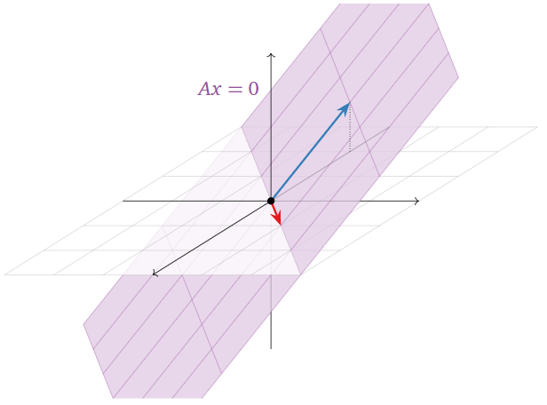
Figure \(\PageIndex{4}\)
Since there were three variables in the above Example \(\PageIndex{4}\), the solution set is a subset of \(\mathbb{R}^3\). Since two of the variables were free, the solution set is a plane.
There is a natural question to ask here: is it possible to write the solution to a homogeneous matrix equation using fewer vectors than the one given in the above recipe? We will see in Example 2.5.3 in Section 2.5 that the answer is no: the vectors from the recipe are always linearly independent, which means that there is no way to write the solution with fewer vectors.
Another natural question is: are the solution sets for inhomogeneuous equations also spans? As we will see shortly, they are never spans, but they are closely related to spans.
There is a natural relationship between the number of free variables and the “size” of the solution set, as follows.
The above examples show us the following pattern: when there is one free variable in a consistent matrix equation, the solution set is a line, and when there are two free variables, the solution set is a plane, etc. The number of free variables is called the dimension of the solution set.
We will develop a rigorous definition, Definition 2.7.2, of dimension in Section 2.7, but for now the dimension will simply mean the number of free variables. Compare with this important note in Section 2.5, Note 2.5.5.
Intuitively, the dimension of a solution set is the number of parameters you need to describe a point in the solution set. For a line only one parameter is needed, and for a plane two parameters are needed. This is similar to how the location of a building on Peachtree Street—which is like a line—is determined by one number and how a street corner in Manhattan—which is like a plane—is specified by two numbers.
Inhomogeneous Systems
Recall that a matrix equation \(Ax=b\) is called inhomogeneous when \(b\neq0\).
What is the solution set of \(Ax=b\text{,}\) where
\[A=\left(\begin{array}{cc}1&-3 \\ 2&-6\end{array}\right)\quad\text{and}\quad b=\left(\begin{array}{c}-3\\-6\end{array}\right)?\nonumber\]
(Compare to this Example \(\PageIndex{4}\), where we solved the corresponding homogeneous equation.)
Solution
We row reduce the associated augmented matrix:
\[\left(\begin{array}{cc|c} 1&-3&-3 \\ 2&-6&-6\end{array}\right) \quad\xrightarrow{\text{RREF}}\quad \left(\begin{array}{cc|c} 1&-3&-3 \\ 0&0&0\end{array}\right).\nonumber\]
This corresponds to the single equation \(x_1 - 3x_2 = -3\). We can write the parametric form as follows:
\[\left\{\begin{array}{rrrrl} x_1 &=& 3x_2 &-& 3\\ x_2 &=& x_2 &+& 0.\end{array}\right.\nonumber\]
We turn the above system into a vector equation:
\[x=\left(\begin{array}{c}x_1 \\ x_2\end{array}\right)=x_2\left(\begin{array}{c}3\\1\end{array}\right)+\left(\begin{array}{c}-3\\0\end{array}\right).\nonumber\]
This vector equation is called the parametric vector form of the solution set. We write the solution set as
\[\text{Span}\left\{\left(\begin{array}{c}3\\1\end{array}\right)\right\}+\left(\begin{array}{c}-3\\0\end{array}\right).\nonumber\]
Here is a picture of the the solution set:
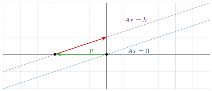
Figure \(\PageIndex{6}\)
In the above Example \(\PageIndex{5}\), the solution set was all vectors of the form
\[x=\left(\begin{array}{c}x_1 \\ x_2\end{array}\right)=x_2\left(\begin{array}{c}3\\1\end{array}\right)+\left(\begin{array}{c}-3\\0\end{array}\right)\nonumber\]
where \(x_2\) is any scalar. The vector \(p = {-3\choose 0}\) is also a solution of \(Ax=b\text{:}\) take \(x_2=0\). We call \(p\) a particular solution.
In the solution set, \(x_2\) is allowed to be anything, and so the solution set is obtained as follows: we take all scalar multiples of \({3\choose 1}\) and then add the particular solution \(p = {-3\choose 0}\) to each of these scalar multiples. Geometrically, this is accomplished by first drawing the span of \({3\choose 1}\text{,}\) which is a line through the origin (and, not coincidentally, the solution to \(Ax=0\)), and we translate, or push, this line along \(p = {-3\choose 0}\). The translated line contains \(p\) and is parallel to \(\text{Span}\{{3\choose 1}\}\text{:}\) it is a translate of a line.
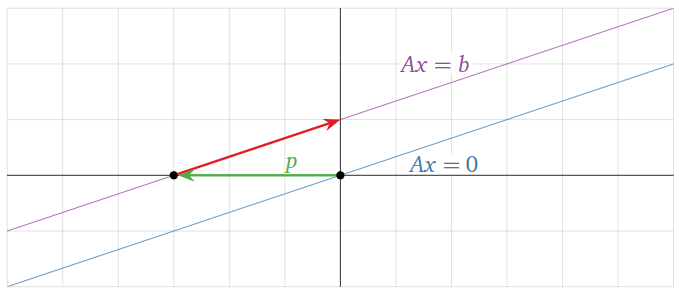
Figure \(\PageIndex{8}\)
What is the solution set of \(Ax=b\text{,}\) where
\[A=\left(\begin{array}{ccc}1&-1&2\\-2&2&-4\end{array}\right)\quad\text{and}\quad b=\left(\begin{array}{c}1\\-2\end{array}\right)?\nonumber\]
(Compare this Example \(\PageIndex{4}\).)
Solution
We row reduce the associated augmented matrix:
\[\left(\begin{array}{ccc|c} 1&-1&2&1 \\ -2&2&-4&-2\end{array}\right) \quad\xrightarrow{\text{RREF}}\quad \left(\begin{array}{cccc}1&-1&2&1 \\ 0&0&0&0\end{array}\right).\nonumber\]
This corresponds to the single equation \(x_1 - x_2 + 2x_3 = 1\). We can write the parametric form as follows:
\[\left\{\begin{array}{rrrrrrl} x_1 &=& x_2 &-& 2x_3 &+& 1\\ x_2 &=& x_2 &{}&{}& +& 0\\ x_3 &=&{}&{}& x_3 &+& 0.\end{array}\right.\nonumber\]
We turn the above system into a vector equation:
\[x=\left(\begin{array}{c}x_1 \\x_2\\x_3\end{array}\right)=x_{2}\left(\begin{array}{c}1\\1\\0\end{array}\right)+x_3\left(\begin{array}{c}-2\\0\\1\end{array}\right)+\left(\begin{array}{c}1\\0\\0\end{array}\right).\nonumber\]
This vector equation is called the parametric vector form of the solution set. Since \(x_2\) and \(x_3\) are allowed to be anything, this says that the solution set is the set of all linear combinations of \(\left(\begin{array}{c}1\\1\\1\end{array}\right)\) and \(\left(\begin{array}{c}-2\\0\\1\end{array}\right)\), translated by the vector \(p=\left(\begin{array}{c}1\\0\\0\end{array}\right)\). This is a plane which contains \(p\) and is parallel to \(\text{Span}\left\{\left(\begin{array}{c}1\\1\\1\end{array}\right),\:\left(\begin{array}{c}-2\\0\\1\end{array}\right)\right\}\text{:}\) it is a translate of a plane. We write the solution set as
\[\text{Span}\left\{\left(\begin{array}{c}1\\1\\1\end{array}\right),\:\left(\begin{array}{c}-2\\0\\1\end{array}\right)\right\} +\left(\begin{array}{c}1\\0\\0\end{array}\right).\nonumber\]
Here is a picture of the solution set:
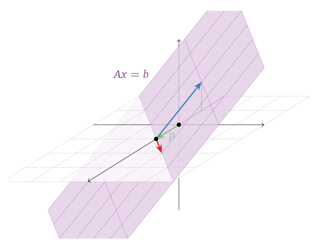
Figure \(\PageIndex{9}\)
In the above Example \(\PageIndex{6}\), the solution set was all vectors of the form
\[x=\left(\begin{array}{c}x_1 \\ x_2 \\ x_3\end{array}\right) =x_2\left(\begin{array}{c}1\\1\\0\end{array}\right)+x_3\left(\begin{array}{c}-2\\0\\1\end{array}\right)+\left(\begin{array}{c}1\\0\\0\end{array}\right).\nonumber\]
where \(x_2\) and \(x_3\) are any scalars. In this case, a particular solution is \(p=\left(\begin{array}{c}1\\0\\0\end{array}\right)\).
In the previous Example \(\PageIndex{6}\) and the Example \(\PageIndex{5}\) before it, the parametric vector form of the solution set of \(Ax=b\) was exactly the same as the parametric vector form of the solution set of \(Ax=0\) (from this Example \(\PageIndex{4}\) and this Example \(\PageIndex{3}\), respectively), plus a particular solution.
If \(Ax=b\) is consistent, the set of solutions to is obtained by taking one particular solution \(p\) of \(Ax=b\text{,}\) and adding all solutions of \(Ax=0\).
In particular, if \(Ax=b\) is consistent, the solution set is a translate of a span.
The parametric vector form of the solutions of \(Ax=b\) is just the parametric vector form of the solutions of \(Ax=0\text{,}\) plus a particular solution \(p\).
It is not hard to see why the key observation \(\PageIndex{3}\) is true. If \(p\) is a particular solution, then \(Ap=b\text{,}\) and if \(x\) is a solution to the homogeneous equation \(Ax=0\text{,}\) then
\[ A(x+p) = Ax + Ap = 0 + b = b, \nonumber \]
so \(x+p\) is another solution of \(Ax=b\). On the other hand, if we start with any solution \(x\) to \(Ax=b\) then \(x-p\) is a solution to \(Ax=0\) since
\[ A(x-p)=Ax-Ap=b-b=0\text{.} \nonumber \]
Row reducing to find the parametric vector form will give you one particular solution \(p\) of \(Ax=b\). But the key observation \(\PageIndex{3}\) is true for any solution \(p\). In other words, if we row reduce in a different way and find a different solution \(p'\) to \(Ax=b\) then the solutions to \(Ax=b\) can be obtained from the solutions to \(Ax=0\) by either adding \(p\) or by adding \(p'\).
What is the solution set of \(Ax=b\text{,}\) where
\[A=\left(\begin{array}{c}1&3&4\\2&-1&2 \\ 1&0&1\end{array}\right)\quad\text{and}\quad b=\left(\begin{array}{c}0\\1\\0\end{array}\right)?\nonumber\]
Solution
We form an augmented matrix and row reduce:
\[\left(\begin{array}{ccc|c} 1&3&4&0 \\ 2&-1&2&1 \\ 1&0&1&0\end{array}\right) \quad\xrightarrow{\text{RREF}}\quad \left(\begin{array}{ccc|c} 1&0&0&-1 \\ 0&1&0&-1 \\ 0&0&1&1\end{array}\right).\nonumber\]
The only solution is \(p=\left(\begin{array}{c}-1\\-1\\1\end{array}\right)\).
According to the key observation \(\PageIndex{3}\), this is supposed to be a translate of a span by \(p\). Indeed, we saw in the first Example \(\PageIndex{1}\) that the only solution of \(Ax=0\) is the trivial solution, i.e., that the solution set is the one-point set \(\{0\}\). The solution set of the inhomogeneous equation \(Ax=b\) is
\[\{0\}+\left(\begin{array}{c}-1\\-1\\1\end{array}\right).\nonumber\]
Note that \(\{0\} = \text{Span}\{0\}\text{,}\) so the homogeneous solution set is a span.
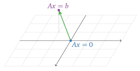
Figure \(\PageIndex{11}\)
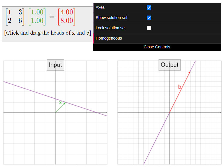
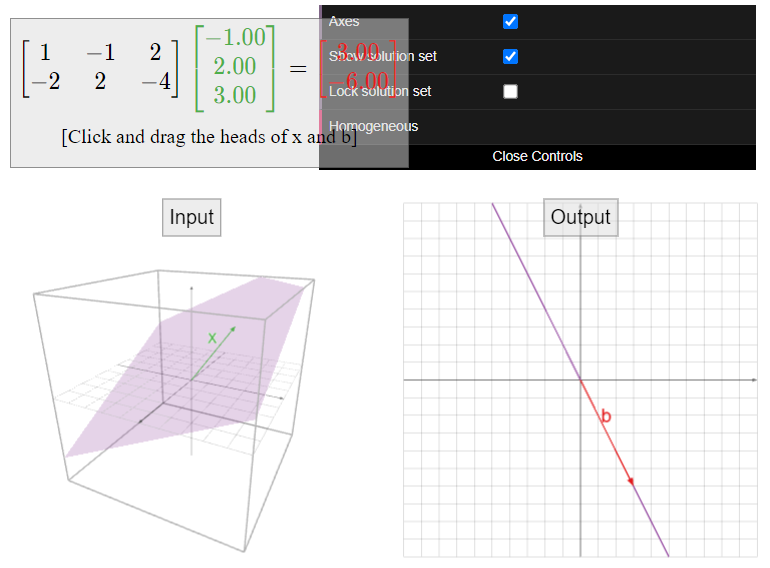
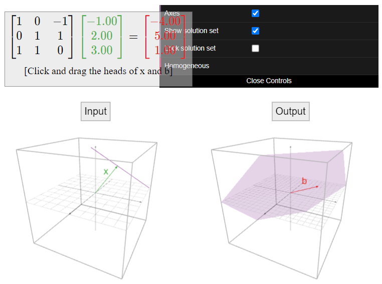
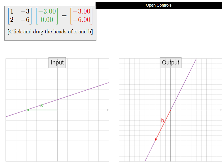
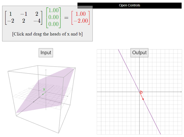
See the interactive figures in the next Subsection Solution Sets and Column Spans for visualizations of the key observation \(\PageIndex{3}\).
As in this important note, when there is one free variable in a consistent matrix equation, the solution set is a line—this line does not pass through the origin when the system is inhomogeneous—when there are two free variables, the solution set is a plane (again not through the origin when the system is inhomogeneous), etc.
Again compare with this important note in Section 2.5, Note 2.5.5.
Solution Sets and Column Spans
To every \(m\times n\) matrix \(A\text{,}\) we have now associated two completely different geometric objects, both described using spans.
- The solution set: for fixed \(b\text{,}\) this is the set of all \(x\) such that \(Ax=b\).
- This is a span if \(b=0\text{,}\) and it is a translate of a span if \(b\neq 0\) (and \(Ax=b\) is consistent).
- It is a subset of \(\mathbb{R}^n\).
- It is computed by solving a system of equations: usually by row reducing and finding the parametric vector form.
- The span of the columns of \(A\): this is the set of all \(b\) such that \(Ax=b\) is consistent.
- This is always a span.
- It is a subset of \(\mathbb{R}^m\).
- It is not computed by solving a system of equations: row reduction plays no role.
Do not confuse these two geometric constructions! In the first the question is which \(x\)’s work for a given \(b\) and in the second the question is which \(b\)’s work for some \(x\).