
1.3: Parametric Form
- Page ID
- 70184

\( \newcommand{\vecs}[1]{\overset { \scriptstyle \rightharpoonup} {\mathbf{#1}} } \)
\( \newcommand{\vecd}[1]{\overset{-\!-\!\rightharpoonup}{\vphantom{a}\smash {#1}}} \)
\( \newcommand{\id}{\mathrm{id}}\) \( \newcommand{\Span}{\mathrm{span}}\)
( \newcommand{\kernel}{\mathrm{null}\,}\) \( \newcommand{\range}{\mathrm{range}\,}\)
\( \newcommand{\RealPart}{\mathrm{Re}}\) \( \newcommand{\ImaginaryPart}{\mathrm{Im}}\)
\( \newcommand{\Argument}{\mathrm{Arg}}\) \( \newcommand{\norm}[1]{\| #1 \|}\)
\( \newcommand{\inner}[2]{\langle #1, #2 \rangle}\)
\( \newcommand{\Span}{\mathrm{span}}\)
\( \newcommand{\id}{\mathrm{id}}\)
\( \newcommand{\Span}{\mathrm{span}}\)
\( \newcommand{\kernel}{\mathrm{null}\,}\)
\( \newcommand{\range}{\mathrm{range}\,}\)
\( \newcommand{\RealPart}{\mathrm{Re}}\)
\( \newcommand{\ImaginaryPart}{\mathrm{Im}}\)
\( \newcommand{\Argument}{\mathrm{Arg}}\)
\( \newcommand{\norm}[1]{\| #1 \|}\)
\( \newcommand{\inner}[2]{\langle #1, #2 \rangle}\)
\( \newcommand{\Span}{\mathrm{span}}\) \( \newcommand{\AA}{\unicode[.8,0]{x212B}}\)
\( \newcommand{\vectorA}[1]{\vec{#1}} % arrow\)
\( \newcommand{\vectorAt}[1]{\vec{\text{#1}}} % arrow\)
\( \newcommand{\vectorB}[1]{\overset { \scriptstyle \rightharpoonup} {\mathbf{#1}} } \)
\( \newcommand{\vectorC}[1]{\textbf{#1}} \)
\( \newcommand{\vectorD}[1]{\overrightarrow{#1}} \)
\( \newcommand{\vectorDt}[1]{\overrightarrow{\text{#1}}} \)
\( \newcommand{\vectE}[1]{\overset{-\!-\!\rightharpoonup}{\vphantom{a}\smash{\mathbf {#1}}}} \)
\( \newcommand{\vecs}[1]{\overset { \scriptstyle \rightharpoonup} {\mathbf{#1}} } \)
\( \newcommand{\vecd}[1]{\overset{-\!-\!\rightharpoonup}{\vphantom{a}\smash {#1}}} \)
\(\newcommand{\avec}{\mathbf a}\) \(\newcommand{\bvec}{\mathbf b}\) \(\newcommand{\cvec}{\mathbf c}\) \(\newcommand{\dvec}{\mathbf d}\) \(\newcommand{\dtil}{\widetilde{\mathbf d}}\) \(\newcommand{\evec}{\mathbf e}\) \(\newcommand{\fvec}{\mathbf f}\) \(\newcommand{\nvec}{\mathbf n}\) \(\newcommand{\pvec}{\mathbf p}\) \(\newcommand{\qvec}{\mathbf q}\) \(\newcommand{\svec}{\mathbf s}\) \(\newcommand{\tvec}{\mathbf t}\) \(\newcommand{\uvec}{\mathbf u}\) \(\newcommand{\vvec}{\mathbf v}\) \(\newcommand{\wvec}{\mathbf w}\) \(\newcommand{\xvec}{\mathbf x}\) \(\newcommand{\yvec}{\mathbf y}\) \(\newcommand{\zvec}{\mathbf z}\) \(\newcommand{\rvec}{\mathbf r}\) \(\newcommand{\mvec}{\mathbf m}\) \(\newcommand{\zerovec}{\mathbf 0}\) \(\newcommand{\onevec}{\mathbf 1}\) \(\newcommand{\real}{\mathbb R}\) \(\newcommand{\twovec}[2]{\left[\begin{array}{r}#1 \\ #2 \end{array}\right]}\) \(\newcommand{\ctwovec}[2]{\left[\begin{array}{c}#1 \\ #2 \end{array}\right]}\) \(\newcommand{\threevec}[3]{\left[\begin{array}{r}#1 \\ #2 \\ #3 \end{array}\right]}\) \(\newcommand{\cthreevec}[3]{\left[\begin{array}{c}#1 \\ #2 \\ #3 \end{array}\right]}\) \(\newcommand{\fourvec}[4]{\left[\begin{array}{r}#1 \\ #2 \\ #3 \\ #4 \end{array}\right]}\) \(\newcommand{\cfourvec}[4]{\left[\begin{array}{c}#1 \\ #2 \\ #3 \\ #4 \end{array}\right]}\) \(\newcommand{\fivevec}[5]{\left[\begin{array}{r}#1 \\ #2 \\ #3 \\ #4 \\ #5 \\ \end{array}\right]}\) \(\newcommand{\cfivevec}[5]{\left[\begin{array}{c}#1 \\ #2 \\ #3 \\ #4 \\ #5 \\ \end{array}\right]}\) \(\newcommand{\mattwo}[4]{\left[\begin{array}{rr}#1 \amp #2 \\ #3 \amp #4 \\ \end{array}\right]}\) \(\newcommand{\laspan}[1]{\text{Span}\{#1\}}\) \(\newcommand{\bcal}{\cal B}\) \(\newcommand{\ccal}{\cal C}\) \(\newcommand{\scal}{\cal S}\) \(\newcommand{\wcal}{\cal W}\) \(\newcommand{\ecal}{\cal E}\) \(\newcommand{\coords}[2]{\left\{#1\right\}_{#2}}\) \(\newcommand{\gray}[1]{\color{gray}{#1}}\) \(\newcommand{\lgray}[1]{\color{lightgray}{#1}}\) \(\newcommand{\rank}{\operatorname{rank}}\) \(\newcommand{\row}{\text{Row}}\) \(\newcommand{\col}{\text{Col}}\) \(\renewcommand{\row}{\text{Row}}\) \(\newcommand{\nul}{\text{Nul}}\) \(\newcommand{\var}{\text{Var}}\) \(\newcommand{\corr}{\text{corr}}\) \(\newcommand{\len}[1]{\left|#1\right|}\) \(\newcommand{\bbar}{\overline{\bvec}}\) \(\newcommand{\bhat}{\widehat{\bvec}}\) \(\newcommand{\bperp}{\bvec^\perp}\) \(\newcommand{\xhat}{\widehat{\xvec}}\) \(\newcommand{\vhat}{\widehat{\vvec}}\) \(\newcommand{\uhat}{\widehat{\uvec}}\) \(\newcommand{\what}{\widehat{\wvec}}\) \(\newcommand{\Sighat}{\widehat{\Sigma}}\) \(\newcommand{\lt}{<}\) \(\newcommand{\gt}{>}\) \(\newcommand{\amp}{&}\) \(\definecolor{fillinmathshade}{gray}{0.9}\)- Learn to express the solution set of a system of linear equations in parametric form.
- Understand the three possibilities for the number of solutions of a system of linear equations.
- Recipe: parametric form.
- Vocabulary word: free variable.
Free Variables
There is one possibility for the row reduced form of a matrix that we did not see in Section 1.2.
Consider the linear system
\[\left\{\begin{array}{rrrrrrc} 2x &+& y &+& 12z &=& 1\\ x &+& 2y &+& 9z &=& -1.\end{array}\right. \nonumber\]
We solve it using row reduction:
\[\begin{aligned} \left(\begin{array}{ccc|c} 2&1&12&1 \\ 1&2&9&-1 \end{array}\right) \quad\xrightarrow{R_1 \longleftrightarrow R_2}\quad & \left(\begin{array}{ccc|c} \color{red}{1}&2&9&-1 \\ 2&1&12&1 \end{array}\right) &&\color{blue}{\text{(Optional)}} \\ {}\quad\xrightarrow{R_2=R_2-2R_1}\quad & \left(\begin{array}{ccc|c} 1&2&9&-1 \\ \color{red}{0} &-3&-6&3 \end{array}\right) &&\color{blue}{\text{(Step 1c)}} \\ {} \quad\xrightarrow{R_2=R_2\div -3}\quad & \left(\begin{array}{ccc|c} 1&2&9&-1 \\ 0&\color{red}{1} &2&-1 \end{array}\right) &&\color{blue}{\text{(Step 2b)}} \\ {} \quad\xrightarrow{R_1=R_1-2R_2}\quad & \left(\begin{array}{ccc|c} 1&\color{red}{0} &5&1 \\ 0&1&2&-1 \end{array}\right) &&\color{blue}{\text{(Step 2c)}}\end{aligned}\]
This row reduced matrix corresponds to the linear system
\[\left\{\begin{array}{rrrrc} x &+& 5z &=& 1\\ y &+& 2z &=& -1.\end{array}\right. \nonumber\]
In what sense is the system solved? We rewrite as
\[\left\{\begin{array}{rrrrc} x &=& 1& -& 5z \\ y &=& -1& -& 2z\end{array}\right. \nonumber\]
For any value of \(z\text{,}\) there is exactly one value of \(x\) and \(y\) that make the equations true. But we are free to choose any value of \(z\).
We have found all solutions: it is the set of all values \(x,y,z\text{,}\) where
\[\left\{\begin{array}{rrrrr} x &=& 1 &-& 5z\\ y &= &-1& -& 2z\\ z& =& {}&{}& z\end{array}\right. \qquad z\text{ any real number.}\nonumber\]
This is called the parametric form for the solution to the linear system. The variable \(z\) is called a free variable.
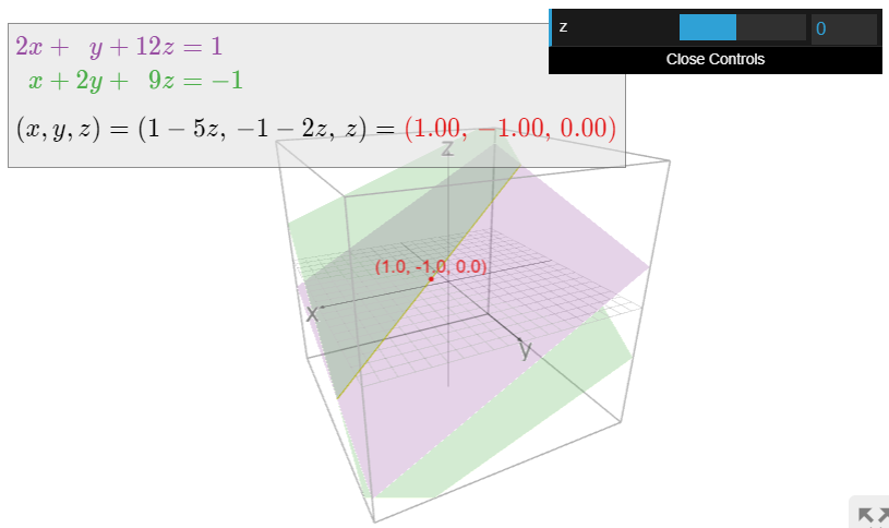
Given the parametric form for the solution to a linear system, we can obtain specific solutions by replacing the free variables with any specific real numbers. For instance, setting \(z=0\) in the last example gives the solution \((x,y,z)=(1,-1,0)\text{,}\) and setting \(z=1\) gives the solution \((x,y,z)=(-4,-3,1)\).
Consider a consistent system of equations in the variables \(x_1,x_2,\ldots,x_n\). Let \(A\) be a row echelon form of the augmented matrix for this system.
We say that \(x_i\) is a free variable if its corresponding column in \(A\) is not a pivot column, Definition 1.2.5 in Section 1.2.
In the above Example, \(\PageIndex{1}\), the variable \(\color{red}z\) was free because the reduced row echelon form matrix was
\[\left(\begin{array}{ccc|c} 1&0&\color{red}{5}&1 \\ 0&1&\color{red}{2}&-1\end{array}\right). \nonumber\]
In the matrix
\[\left(\begin{array}{cccc|c} 1&\color{red}{\star} &0&\color{blue}{\star} &\star \\ 0&\color{red}{0}&1&\color{blue}{\star}&\star \end{array}\right),\nonumber\]
the free variables are \(\color{red}x_2\) and \(\color{blue}x_4\). (The augmented column is not free because it does not correspond to a variable.)
The parametric form of the solution set of a consistent system of linear equations is obtained as follows.
- Write the system as an augmented matrix.
- Row reduce to reduced row echelon form.
- Write the corresponding (solved) system of linear equations.
- Move all free variables to the right hand side of the equations.
Moving the free variables to the right hand side of the equations amounts to solving for the non-free variables (the ones that come pivot columns) in terms of the free variables. One can think of the free variables as being independent variables, and the non-free variables being dependent.
The solution set of the system of linear equations
\[\left\{\begin{array}{rrrrrrr} 2x &+& y &+& 12z &=& 1\\ x &+& 2y &+& 9z &=& -1 \end{array}\right. \nonumber\]
is a line in \(\mathbb{R}^3\text{,}\) as we saw in Example \(\PageIndex{1}\). These equations are called the implicit equations for the line: the line is defined implicitly as the simultaneous solutions to those two equations.
The parametric form
\[\left\{\begin{array}{rrrrc} x &=& 1 &-& 5z\\ y &=& -1 &-& 2z.\end{array}\right.\nonumber\]
can be written as follows:
\[ (x,\,y,\,z) = (1-5z,\,-1-2z,\,z) \qquad \text{$z$ any real number.} \nonumber \]
This called a parameterized equation for the same line. It is an expression that produces all points of the line in terms of one parameter, \(z\).
One should think of a system of equations as being an implicit equation for its solution set, and of the parametric form as being the parameterized equation for the same set. The parameteric form is much more explicit: it gives a concrete recipe for producing all solutions.
You can choose any value for the free variables in a (consistent) linear system.
Free variables come from the columns without pivots in a matrix in row echelon form.
Suppose that the reduced row echelon form of the matrix for a linear system in four variables \(x_1,x_2,x_3,x_4\) is
\[\left(\begin{array}{cccc|c} 1&\color{red}{0}&0&\color{blue}{3}&2 \\ 0&\color{red}{0}&1&\color{blue}{4}&-1\end{array}\right).\nonumber\]
The free variables are \(\color{red}x_2\) and \(\color{blue}x_4\text{:}\) they are the ones whose columns are not pivot columns.
This translates into the system of equations
\[\left\{\begin{array}{rrrrrrrrr} x_1 &{}&{}&{}&{}&+& 3x_4 &=& 2 \\ {}&{}&{}&{}& x_3 &+& 4x_4 &=& -1\end{array}\right. \quad\xrightarrow{\text{parametric form}}\quad \left\{\begin{array}{rrrrc} x_1 &=& 2 &-& 3x_4\\ x_3 &=& -1 &-& 4x_4. \end{array}\right.\nonumber\]
What happened to \(x_2\text{?}\) It is a free variable, but no other variable depends on it. The general solution to the system is
\[ (x_1,\,x_2,\,x_3,\,x_4) = (2-3x_4,\,x_2,\,-1-4x_4,\,x_4), \nonumber \]
for any values of \(x_2\) and \(x_4\). For instance, \((2,0,-1,0)\) is a solution (with \(x_2=x_4=0\)), and \((5,1,3,-1)\) is a solution (with \(x_2=1, x_4=-1\)).
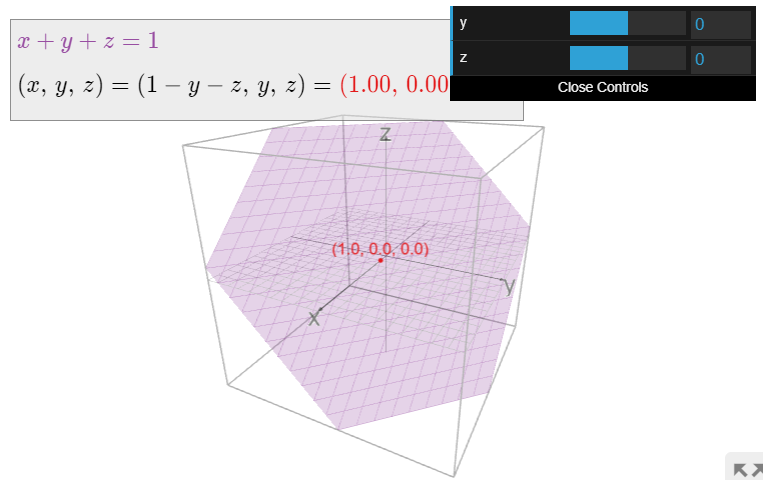
The system of one linear equation
\[ x + y + z = 1 \nonumber \]
comes from the matrix
\[\left(\begin{array}{ccc|c} 1&1&1&1\end{array}\right),\nonumber\]
which is already in reduced row echelon form. The free variables are \(y\) and \(z\). The parametric form for the general solution is
\[ (x,\,y,\,z) = (1 - y - z,\,y,\,z) \nonumber \]
for any values of \(y\) and \(z\). This is the parametric equation for a plane in \(\mathbb{R}^3\).
Number of Solutions
There are three possibilities for the reduced row echelon form of the augmented matrix of a linear system.
- The last column is a pivot column. In this case, the system is inconsistent. There are zero solutions, i.e., the solution set is empty. For example, the matrix
\[\left(\begin{array}{cc|c} 1&0&\color{red}{0} \\ 0&1&\color{red}{0} \\ 0&0&\color{red}{1}\end{array}\right)\nonumber\]
comes from a linear system with no solutions. - Every column except the last column is a pivot column. In this case, the system has a unique solution. For example, the matrix
\[\left(\begin{array}{ccc|c} 1&0&0&a \\ 0&1&0&b \\ 0&0&1&c \end{array}\right)\nonumber\]
tells us that the unique solution is \((x,y,z)=(a,b,c)\). - The last column is not a pivot column, and some other column is not a pivot column either. In this case, the system has infinitely many solutions, corresponding to the infinitely many possible values of the free variable(s). For example, in the system corresponding to the matrix
\[\left(\begin{array}{cccc|c} 1&\color{red}{-2}&0&\color{blue}{3}&1\\ 0&\color{red}{0}&1&\color{blue}{4}&-1\end{array}\right),\nonumber\]
any values for \(\color{red}x_2\) and \(\color{blue}x_4\) yield a solution to the system of equations.