16.2: Pick and Place

# Here are some libraries you may need to use
%matplotlib inline
import matplotlib.pylab as plt
import numpy as np
import sympy as sym
import math
sym.init_printing()

Consider the robot depicted in the following image.

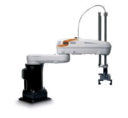
This style of robot is often called a “pick-and-place” robot. It has two motors that rotate around the z-axis to move the end effector in the \(x−y\) plane; one “linear actuator” which moves up-and-down in the \(z\)-direction; and then finally a third rotating “wrist” joint that turns the “hand” of the robot. Let’s model our robot using the following system diagram:

Note

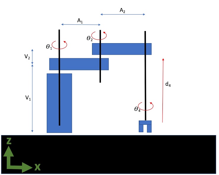
The origin for this robot is located at the base of the first “tower” and is in-line with the first joint. The \(x\)-direction goes from the origin to the right and the \(z\)-axis goes from the origin upwards.

This is a little more tricky than the 2D case where everything was rotating around the axes that projects out of the \(x−y\) plane.

In 2D we only really worry about one axis of rotation. However in 3D we can rotate around the \(x\), \(y\), and \(z\) axis. The following are the 3D transformation matrices that combine rotation and translations:

X-Axis rotation

\[\begin{split}
\left[ \begin{matrix}
x' \\
y' \\
z' \\
1
\end{matrix}
\right]
=
\left[ \begin{matrix}
1 & 0 & 0 & dx \\
0 & cos(q) & -sin(q) & dy \\
0 & sin(q) & cos(q) & dz \\
0 & 0 & 0 & 1
\end{matrix}
\right]
\left[ \begin{matrix}
x \\
y \\
z \\
1
\end{matrix}
\right]
\end{split} \nonumber \]

Y-Axis rotation

\[\begin{split}
\left[ \begin{matrix}
x' \\
y' \\
z' \\
1
\end{matrix}
\right]
=
\left[ \begin{matrix}
cos(q) & 0 & sin(q) & dx \\
0 & 1 & 0 & dy \\
-sin(q) & 0 & cos(q) & dz \\
0 & 0 & 0 & 1
\end{matrix}
\right]
\left[ \begin{matrix}
x \\
y \\
z \\
1
\end{matrix}
\right]
\end{split} \nonumber \]

Z-Axis rotation

\[\begin{split}
\left[ \begin{matrix}
x' \\
y' \\
z' \\
1
\end{matrix}
\right]
=
\left[ \begin{matrix}
cos(q) & -sin(q) & 0 & dx \\
sin(q) & cos(q) & 0 & dy \\
0 & 0 & 1 & dz \\
0 & 0 & 0 & 1
\end{matrix}
\right]
\left[ \begin{matrix}
x \\
y \\
z \\
1
\end{matrix}
\right]
\end{split} \nonumber \]

Question (a)

Construct a joint transformation matrix called \(J_1\), which represents a coordinate system that is located at the top of the first “tower” (robot’s sholder) and moves by rotating around the \(z\)-axis by \(\theta_1\) degrees. Represent your matrix using sympy and the provided symbols:

#Use the following symbols

q1,q2,d4,q4,v1,v2,a1,a2 = sym.symbols('\Theta_1, \Theta_2, d_4, \Theta_4, V_1, V_2,A_1,A_2', negative=False)

#put your answer here
q1

Question (b)

Construct a joint transformation matrix called \(J_2\), which represents a coordinate system that is located at the “elbow” joint between the two rotating arms and rotates with the second arm around the \(z\)-axis by \(\theta_2\) degrees. Represent your matrix using sympy and the symbols provided in question a:

#put your answer here

Question (c)

Construct a joint transformation matrix called \(J_3\), which represents a coordinate translation from the “elbow” joint all the way to the horizontal end of the robot arm above the wrist joint. Note: there is no rotation in this transformation. Represent your matrix using sympy and the symbols provided in question a:

#put your answer here

Question (d)

Construct a joint transformation matrix called \(J_4\), which represents a coordinate system that is located at the tip of the robot’s “hand” and rotates around the \(z\)-axis by \(\theta_4\). This one is a little different, the configuration is such that the hand touches the table when \(d_4=0\) so the translation component for the matrix in the z axis is \(d_4−V_1−V_2\).

#put your answer here

Question

Rewrite the joint transformation matrices from questions a - d as numpy matrices with discrete (instead of symbolic) values. Plug in your transformations in the code below and use this to simulate the robot:

from ipywidgets import interact
from mpl_toolkits.mplot3d import Axes3D

def Robot_Simulator(theta1=0,theta2=-0,d4=0,theta4=0):

    #Convert from degrees to radians
    q1 = theta1/180 * math.pi
    q2 = theta2/180 * math.pi
    q4 = theta4/180 * math.pi

    #Define robot geomitry
    V1 = 4 
    V2 = 0
    A1 = 2 
    A2 = 2 

    #Define your transfomraiton matrices here. 
    J1 = np.matrix([[1, 0, 0, 0 ], 
                    [0, 1, 0, 0 ], 
                    [0, 0, 1, 0],
                    [0, 0, 0, 1]])

    J2 = np.matrix([[1, 0, 0, 0 ], 
                    [0, 1, 0, 0 ], 
                    [0, 0, 1, 0],
                    [0, 0, 0, 1]])

    J3 = np.matrix([[1, 0, 0, 0 ], 
                    [0, 1, 0, 0 ], 
                    [0, 0, 1, 0],
                    [0, 0, 0, 1]])

    J4 = np.matrix([[1, 0, 0, 0 ], 
                    [0, 1, 0, 0 ], 
                    [0, 0, 1, 0],
                    [0, 0, 0, 1]])

    
    #Make the rigid end effector
    p = np.matrix([[-0.5,0,0, 1], [-0.5,0,0.5,1], [0.5,0,0.5, 1], [0.5,0,0,1],[0.5,0,0.5, 1], [0,0,0.5,1], [0,0,V1+V2,1]]).T
    
    #Propogate and add joint points though the simulation
    p = np.concatenate((J4*p, np.matrix([0,0,0,1]).T), axis=1 )
    p = np.concatenate((J3*p, np.matrix([0,0,0,1]).T), axis=1 )
    p = np.concatenate((J2*p, np.matrix([0,0,0,1]).T), axis=1 )
    p = np.concatenate((J1*p, np.matrix([0,0,0,1]).T), axis=1 )
        
    fig = plt.figure()
    ax = fig.add_subplot(111, projection='3d')

    ax.scatter(p[0,:].tolist()[0],(p[1,:]).tolist()[0], (p[2,:]).tolist()[0], s=20, facecolors='blue', edgecolors='r')
    ax.scatter(0,0,0, s=20, facecolors='r', edgecolors='r')
    ax.plot(p[0,:].tolist()[0],(p[1,:]).tolist()[0], (p[2,:]).tolist()[0])
    ax.set_xlim([-5,5])
    ax.set_ylim([-5,5])
    ax.set_zlim([0,6])
    ax.set_xlabel('x-axis')
    ax.set_ylabel('y-axis')    
    ax.set_zlabel('z-axis') 

    plt.show()
    
target = interact(Robot_Simulator, theta1=(-180,180), theta2=(-180,180), d4=(0,6), theta4=(-180,180)); ##TODO: Modify this line of code

theta1

0

theta2

0

d4

0

theta4

0

Question

Can we change the order of the transformation matrices? Why? You can try and see what happens.