20.2: Introduction to Markov Models

%matplotlib inline
import matplotlib.pylab as plt
import numpy as np
import sympy as sym
sym.init_printing(use_unicode=True)
from urllib.request import urlretrieve

urlretrieve('https://raw.githubusercontent.com/colbrydi/jupytercheck/master/answercheck.py', 
            'answercheck.py');

In probability theory, a Markov model is a stochastic model used to model randomly changing systems. It is assumed that future states depend only on the current state, not on the events that occurred before it.

A diagram representing a two-state Markov process, with the states labelled E and A. Via Wikipedia

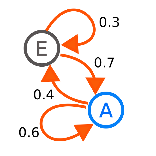
Each number represents the probability of the Markov process changing from one state to another state, with the direction indicated by the arrow. For example, if the Markov process is in state A, then the probability it changes to state E is 0.4, while the probability it remains in state A is 0.6.

The above state model can be represented by a transition matrix.

\[\begin{split}\begin{array}{cc}
& \text{Current State} \\
P = &
\begin{bmatrix}
p_{A\rightarrow A} & p_{E\rightarrow A} \\
p_{A\rightarrow E} & p_{E\rightarrow E}
\end{bmatrix}
\end{array}
\text{Next state}\end{split} \nonumber \]

In other words we can write the above as follows

A = np.matrix([[0.6, 0.7],[0.4, 0.3]])
sym.Matrix(A)

Notice how the columns in the matrix all add to one. This is because all of the transition probabilities out of a matrix must add to 100 percent.

Now, consider the following house map with cats in each room…

At each time step, there is an equal probability of a cat staying in their current room or moving to a new room. If a cat chooses to leave a room, then there is an equal chance of that cat picking any of the doors in the room to leave.

Do This

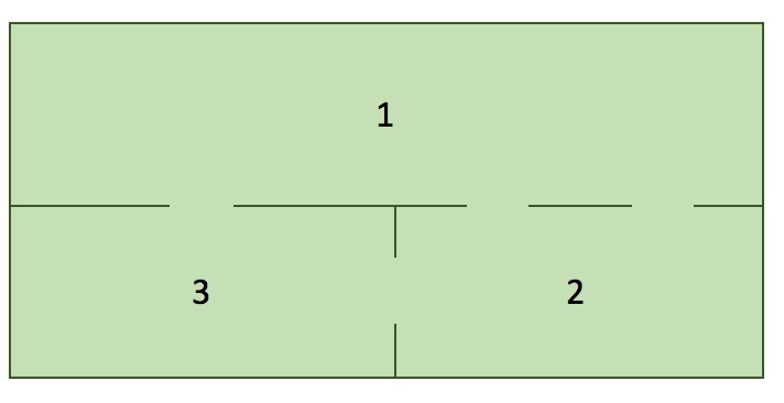
Try to draw a Markov chain (Markov matrix) for the above system of equations. Be prepared to share your diagram with the class.

A Markov chain can be represented as a Markov transition model of the form \(Ax=b\). Where \(A\) is your probability tranisition matrix (often represented as a \(P\) instead of an \(A\)). \(x\) is the state before the transition and \(b\) is the state after the transition.

Question

Generate a Markov transition model represented as a matrix \(P\) of the form:

\[
\begin{array}{ccc}
& \text{Current Room} \\
P = &
\begin{bmatrix}
p_{11} & p_{12} & p_{13} \\
p_{21} & p_{22} & p_{23} \\
p_{31} & p_{32} & p_{33}
\end{bmatrix}
\end{array}
\text{Next Room} \nonumber \]

Where \(p_{ij}\) are probability transitions of the cat moving between rooms (from room \(j\) to room \(i\)):

##put your answer here

from answercheck import checkanswer

checkanswer.matrix(P,'1001a6fa07727caf8ce05226b765542c');

Question

Let’s assume that the system starts with; 6 cats in room 1, 15 cats in room 2, and 3 cats in room 3. How many cats will be in each room after one time step (Store the values in a vector called current_state)?

#Put your answer to the above question here.

from answercheck import checkanswer

checkanswer.vector(current_state,'98d5519be82a0585654de5eda3a7f397');

Question

The following code will plot the number of cats as a function of time (\(t\)). When this system converges, what is the steady state?

#Define Start State
room1 = [6]
room2 = [15]
room3 = [3]

current_state = np.matrix([room1, room2, room3])

for i in range(10):
    #update Current State
    current_state = P*current_state
    
    #Store history for each room
    room1.append(current_state[0])
    room2.append(current_state[1])
    room3.append(current_state[2])
    
plt.plot(room1, label="room1");
plt.plot(room2, label="room2");
plt.plot(room3, label="room3");
plt.legend();
print(current_state)

Question

Calculate the eigenvalues and eigenvectors of your \(P\) transition matrix.

##put your answer here

Do This

Make a new vector called steadystate from the eigenvector of your \(P\) matrix with a eigenvalue of 1.

## Put your answer here

Since the steadystate vectors represent long term probabilities, they should sum to one (1). However, most programming libraries (ex. numpy and sympy) return “normalized” eigenvectors to length of 1 (i.e. norm(e)==1).

Do This

Correct for the normalization by multiplying the steadystate eigenvector by a constant such that the sum of the vector elements add to 1.

#Put your answer here

Do This

Think about the cats problem, because one cat has to be in one of the three rooms. That means, the total number of cats will not change. If we add the number of cats at all rooms together, this number has to be the same. Therefore, if we start will 6+15+3=24 cats, there are also 24 cats at the steadystate. Modify the steadystate to make sure the total number of cats is 24.

Question

Why does the sum of the numbers at every stage remain the same?