5.1: Limits

The idea of a limit is the cornerstone of calculus. It is somewhat subtle, which is why, although it was implicit in the work of Archimedes \(^{1}\), and essential to a proper understanding of Zeno’s paradoxes, it took two thousand years to be understood fully. Calculus was developed in the \(17^{\text {th }}\) century by Newton and Leibniz with a somewhat cavalier approach to limits; it was not until the \(19^{\text {th }}\) century that a rigorous definition of limit was given, by Cauchy.

In Section \(5.1\) we define limits, and prove some elementary properties. In Section \(5.2\) we discuss continuous functions, and in Section \(5.3\) we look at limits of sequences of functions.

Limits

Given a real function \(f: X \rightarrow \mathbb{R}\), the intuitive idea of the statement \[\lim _{x \rightarrow a} f(x)=L\] is that, as \(x\) gets closer and closer to \(a\), the values of \(f(x)\) get closer and closer to \(L\). Making this notion precise is not easy - try to write down a mathematical definition now, before you read any further.

The idea behind the definition is to give a sequence of guarantees. Imagine yourself as an attorney, trying to defend the claim (5.1). For concreteness, let us fix \(g(x)=\frac{\sin (x)}{x}\), and try to defend the claim that \[\lim _{x \rightarrow 0} g(x)=1\] \({ }^{1}\) Archimedes (287-212 BC) calculated the area under a parabola (what we would now call \(\int_{0}^{1} x^{2} d x\) ) by calculating the area of the rectangles of width \(1 / N\) under the parabola and letting \(N\) tend to infinity. This is identical to the modern approach of finding an integral by taking a limit of Riemann sums.

FIGURE 5.3. Plot of \(\sin (x) / x\)

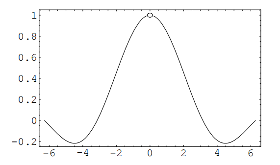
The skeptical judge asks "Can you guarantee that \(g(x)\) is within .1 of 1 ?"

"Yes, your honor, provided that \(|x|<.7\)."

"Hmm, well can you guarantee that \(g(x)\) is within \(.01\) of 1 ?"

"Yes, your honor, provided that \(|x|<.2 . "\)

And so it goes. If, for every possible tolerance the judge poses, you can find a precision (i.e. an allowable deviation of \(x\) from \(a\) ) that guarantees that the difference between the function value and the limit is within the allowable tolerance, then you can successfully defend the claim.

EXERCISE. Now try to give a mathematical definition of a limit, without reading any further.

We shall start with the case that the function is defined on an open interval.

DEFINITION. Limit, \(\lim _{x \rightarrow a} f(x)\) Let \(I\) be an open interval and \(a\) some point in \(I\). Let \(f\) be a real-valued function defined on \(I \backslash\{a\}\). (It doesn’t matter whether \(f\) is defined at \(a\) or not). Then we say \[\lim _{x \rightarrow a} f(x)=L\] (in words, "the limit as \(x\) tends to \(a\) of \(f(x)\) is \(L\) ") if, for every \(\varepsilon>0\), there exists \(\delta>0\), so that \[0<|x-a|<\delta \quad \Longrightarrow \quad|f(x)-L|<\varepsilon\]

FIGURE 5.5. One choice of \(\delta\) for a given \(\varepsilon\)

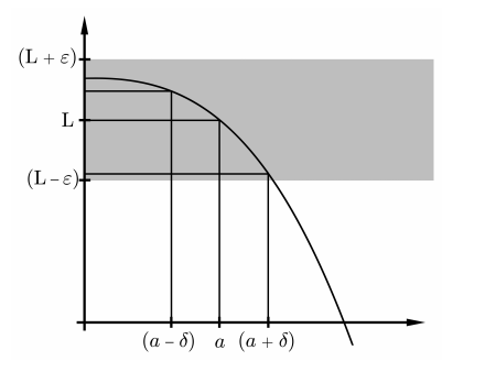
The condition \(0<|x-a|<\delta\) means we exclude \(x=a\) from consideration. Limits are about the behavior of a function near the point, not at the point. For a function like \(g(x)=\sin (x) / x\), the value at 0 is undefined; nevertheless \(\lim _{x \rightarrow 0} g(x)\) exists, and is the same as \(\lim _{x \rightarrow 0}\) of the function \[h(x)=\left\{\begin{array}{cc} \sin (x) / x & x \neq 0 \\ 5 & x=0 . \end{array}\right.\] REMARK. The use of \(\varepsilon\) for the allowable error and \(\delta\) for the corresponding precision required is hallowed by long usage. Mathematicians need all the convenient symbols they can find. The Greek alphabet has long been used as a supplement to the Roman alphabet in Western mathematics, and you need to be familiar with it (see Appendix A for the Greek alphabet). The main point to note in the definition is the order of the quantifiers: \(\forall \varepsilon, \exists \delta\). What would it mean to say \[(\exists \delta>0)(\forall \varepsilon>0) \quad[0<|x-a|<\delta \quad \Longrightarrow \quad|f(x)-L|<\varepsilon] ?\] To talk comfortably about limits, it helps to have some words that describe inequalities (5.4). Let us say that the \(\varepsilon\)-neighborhood of \(L\) is the set of points within \(\varepsilon\) of \(L\), i.e. the interval \((L-\varepsilon, L+\varepsilon)\). The punctured \(\delta\)-neighborhood of \(a\) is the set of points within \(\delta\) of \(a\), excluding \(a\) itself, i.e. \((a-\delta, a) \cup(a, a+\delta)\). When we speak of \(\varepsilon\)-neighborhoods and punctured \(\delta\)-neighborhoods, we always assume that \(\varepsilon\) and \(\delta\) are positive, so that the neighborhoods are non-empty.

Then the definition of limit can be worded as "every \(\varepsilon\)-neighborhood of \(L\) has an inverse image under \(f\) that contains some punctured \(\delta\) neighborhood of \(a\) ".

REMARK. We can revisit our court-room analogy, and say that to prove that \(f\) has limit \(L\) at \(a\), we need a strategy that produces a workable \(\delta\) for any \(\varepsilon\). So a proof is essentially a function \(F\) that takes any positive \(\varepsilon\) and spits out a positive \(\delta=F(\varepsilon)\) for which (5.4) works.

EXAMPLE 5.6. Let \(f(x)=5 x+2\). Prove \(\lim _{x \rightarrow 3} f(x)=17\).

Let \(\varepsilon>0\). We want to find a \(\delta>0\) so that the punctured \(\delta\) neighborhood of 3 is mapped into the \(\varepsilon\)-neighborhood of 17 .

FIGURE 5.7. Relationship between \(\delta\) and \(\varepsilon\)

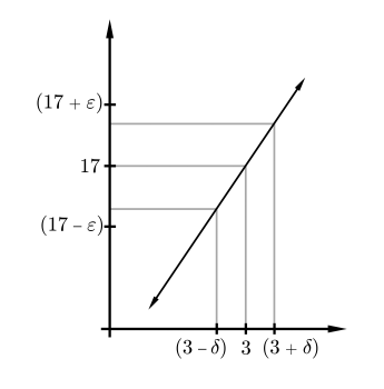
Taking \(\delta=\varepsilon / 5\) will work, as will any smaller choice of \(\delta\). Indeed, if \(0<|x-3|<\delta\), then \(|f(x)-17|<5 \delta=\varepsilon\).

EXAMPLE 5.8. This time, let \(g(x)=55 x+2\). To prove \(\lim _{x \rightarrow 3} g(x)=\) 167 , we must take \(\delta \leq \varepsilon / 55\).

If two functions \(f\) and \(g\) both have limits at the point \(a\), then so do all the algebraic combinations \(f+g, f-g, f \cdot g\) and \(c f\) for \(c\) a constant. The quotient \(f / g\) also has a limit at \(a\), provided \(\lim _{x \rightarrow a} g(x) \neq 0\). Moreover, these limits are what you would expect.

THEOREM 5.9. Suppose \(f\) and \(g\) are functions on an open interval \(I\), and at the point \(a\) in \(I\) both \(\lim _{x \rightarrow a} f(x)\) and \(\lim _{x \rightarrow a} g(x)\) exist. Let \(c\) be any real number. Then \[\begin{aligned} \text { (i) } \lim _{x \rightarrow a}[f(x)+g(x)] &=\lim _{x \rightarrow a} f(x)+\lim _{x \rightarrow a} g(x) \\ \text { (ii) } \lim _{x \rightarrow a}[f(x)-g(x)] &=\lim _{x \rightarrow a} f(x)-\lim _{x \rightarrow a} g(x) \\ \text { (iii) } \quad \lim _{x \rightarrow a} c f(x) &=c\left[\lim _{x \rightarrow a} f(x)\right] \\ (i v) \quad \lim _{x \rightarrow a}[f(x) g(x)] &=\left[\lim _{x \rightarrow a} f(x)\right] \cdot\left[\lim _{x \rightarrow a} g(x)\right] \\ \text { (v) } \quad \lim _{x \rightarrow a} \frac{f(x)}{g(x)} &=\frac{\lim _{x \rightarrow a} f(x)}{\lim _{x \rightarrow a} g(x)}, \quad \text { provided } \lim _{x \rightarrow a} g(x) \neq 0 . \end{aligned}\] DiscuSsion. How do we go about proving a theorem like this? Well, to start with, don’t be intimidated by its length. Let’s start on part (i). We only have the definition of limit to work with, so we only have one strategic option: prove directly that the definition is satisfied.

PROOF OF (i). Let \(L_{1}\) and \(L_{2}\) be the limits of \(f\) and \(g\) respectively at \(a\). Let \(\varepsilon\) be an arbitrary positive number. We must find a \(\delta>0\) so that \[0<|x-a|<\delta \quad \Longrightarrow \quad\left|f(x)+g(x)-\left(L_{1}+L_{2}\right)\right|<\varepsilon .\] The key idea, common to many limit arguments, is to use the observation that \[\left|f(x)+g(x)-\left(L_{1}+L_{2}\right)\right| \leq\left|f(x)-L_{1}\right|+\left|g(x)-L_{2}\right| .\] This is an application of the so-called triangle inequality, which you are asked later to prove (Lemma 5.14). It is the assertion that for any real numbers \(c\) and \(d\), we have \[|c+d| \leq|c|+|d| .\] (What values of \(c\) and \(d\) yield (5.10)?) So if we can make both \(\left|f(x)-L_{1}\right|\) and \(\left|g(x)-L_{2}\right|\) small, then Inequality (5.10) forces \[\left|f(x)+g(x)-\left(L_{1}+L_{2}\right)\right|\] to be small too, which is what we want.

Since \(f\) and \(g\) have limits \(L_{1}\) and \(L_{2}\) at \(a\), we know that there exist positive numbers \(\delta_{1}\) and \(\delta_{2}\) such that \[\begin{array}{lll} 0<|x-a|<\delta_{1} & \Longrightarrow & \left|f(x)-L_{1}\right|<\varepsilon \\ 0<|x-a|<\delta_{2} & \Longrightarrow & \left|g(x)-L_{2}\right|<\varepsilon \end{array}\] If \(|x-a|\) is less than both \(\delta_{1}\) and \(\delta_{2}\), then both inequalities are satisfied, and we get \[\left|f(x)+g(x)-\left(L_{1}+L_{2}\right)\right| \leq\left|f(x)-L_{1}\right|+\left|g(x)-L_{2}\right| \leq \varepsilon+\varepsilon .\] This isn’t quite good enough; we want the left-hand side of (5.11) to be bounded by \(\varepsilon\), not \(2 \varepsilon\). We are saved, however, by the requirement that for any positive number \(\eta\), we can guarantee that \(f\) and \(g\) are in an \(\eta\)-neighborhood of \(L_{1}\) and \(L_{2}\), respectively. In particular, let \(\eta\) be \(\varepsilon / 2\). Since \(f\) and \(g\) have limits at \(a\), there are positive numbers \(\delta_{3}\) and \(\delta_{4}\) so that \[\begin{array}{lll} 0<|x-a|<\delta_{3} & \Longrightarrow & \left|f(x)-L_{1}\right|<\frac{\varepsilon}{2} \\ 0<|x-a|<\delta_{4} & \Longrightarrow & \left|g(x)-L_{2}\right|<\frac{\varepsilon}{2} . \end{array}\] So we set \(\delta\) equal to the smaller of \(\delta_{3}\) and \(\delta_{4}\), and we get \[\begin{aligned} &0<|x-a|<\delta \Longrightarrow \\ &\quad\left|f(x)+g(x)-\left(L_{1}+L_{2}\right)\right| \leq\left|f(x)-L_{1}\right|+\left|g(x)-L_{2}\right|<\varepsilon, \end{aligned}\] as required. ExERCISE. Explain in words how the preceding proof worked. In short-hand, one could say that if \(F_{1}\) and \(F_{2}\) are strategies for proving \(\lim _{x \rightarrow a} f(x)=L_{1}\) and \(\lim _{x \rightarrow a} g(x)=L_{2}\) respectively, then \[F=\min \left\{F_{1}\left(\frac{\varepsilon}{2}\right), F_{2}\left(\frac{\varepsilon}{2}\right)\right\}\] is a strategy for proving \(\lim _{x \rightarrow a} f(x)+g(x)=L_{1}+L_{2}\).

Discussion. What next? We could prove (ii) in a similar way, but mathematicians like shortcuts. Notice that if we prove (iii) and let \(c=-1\), then we can apply (i) to \(f+(-g)\) and get (ii) that way. Moreover, (iii) is just a special case of (iv), if we know that the constant function \(g(x)=c\) has the limit \(c\) at every point. So let us prove (iv) next.

PROOF OF (iv). Again, let \(\varepsilon\) be an arbitrary positive number. We must find a \(\delta>0\) so that \[0<|x-a|<\delta \quad \Longrightarrow \quad\left|f(x) g(x)-\left(L_{1} L_{2}\right)\right|<\varepsilon .\] It is not quite clear how close \(f\) and \(g\) have to be to \(L_{1}\) and \(L_{2}\) to get that their product is close enough to \(L_{1} L_{2}\), so let’s play it safe by not choosing yet. For every \(\varepsilon_{1}, \varepsilon_{2}>0\), we know there exist \(\delta_{1}, \delta_{2}>0\) such that \[\begin{array}{lll} 0<|x-a|<\delta_{1} & \Longrightarrow & \left|f(x)-L_{1}\right|<\varepsilon_{1} \\ 0<|x-a|<\delta_{2} & \Longrightarrow & \left|g(x)-L_{2}\right|<\varepsilon_{2} \end{array}\] Now we use the second common trick in proving the existence of limits: add and subtract the same quantity so that one can factor. \[\begin{aligned} \left|f(x) g(x)-L_{1} L_{2}\right| &=\left|f(x) g(x)-L_{1} g(x)+L_{1} g(x)-L_{1} L_{2}\right| \\ & \leq\left|f(x) g(x)-L_{1} g(x)\right|+\left|L_{1} g(x)-L_{1} L_{2}\right| \\ & \leq\left|f(x)-L_{1}\right||g(x)|+\left|g(x)-L_{2}\right|\left|L_{1}\right| \cdot \quad(5.1 \end{aligned}\] Now if both summands on the last line can be made less than \(\varepsilon / 2\), we win. The second term is easy: we choose \[\varepsilon_{2}=\frac{\varepsilon}{2\left|L_{1}\right|+1} .\] Then there is a \(\delta_{2}\) so that \[\begin{aligned} 0<|x-a|<\delta_{2} & \Longrightarrow \quad\left|g(x)-L_{2}\right| &<\varepsilon_{2} \\ & \Longrightarrow \quad\left|g(x)-L_{2}\right|\left|L_{1}\right| &<\frac{\varepsilon\left|L_{1}\right|}{2\left|L_{1}\right|+1}<\frac{\varepsilon}{2} \end{aligned}\] (If \(L_{1} \neq 0\), we could have chosen \(\varepsilon_{2}=\frac{\varepsilon}{2\left|L_{1}\right|}\); we added 1 to the denominator just so we did not have to consider the two cases separately.)

What about the first summand in (5.12), the term \(\left|f(x)-L_{1}\right||g(x)|\) ? First let us get some bound on how big \(|g|\) can be. We know that if \(0<|x-a|<\delta_{2}\), then \(\left|g(x)-L_{2}\right|<\varepsilon /\left(2\left|L_{1}\right|+1\right)\), so \[|g(x)|<\left|L_{2}\right|+\frac{\varepsilon}{2\left|L_{1}\right|+1}=: M .\] If we let \(\varepsilon_{1}=\varepsilon /(2 M)\), we know that there exists \(\delta_{1}>0\) so that \[0<|x-a|<\delta_{1} \quad \Longrightarrow \quad\left|f(x)-L_{1}\right||g(x)|<\varepsilon_{1}|g(x)| .\] Finally, we let \(\delta=\min \left(\delta_{1}, \delta_{2}\right)\). For \(0<|x-a|<\delta\), both summands in (5.12) are less than \(\varepsilon / 2\) : the second summand because \(\delta \leq \delta_{2}\), and the first because when \(0<|x-a|<\delta\), Inequality \(5.13\) is strengthened to \[\left|f(x)-L_{1}\right||g(x)|<\varepsilon_{1}|g(x)|<\varepsilon_{1} M=\varepsilon / 2 .\] Therefore, for \(0<|x-a|<\delta\), we have \(\left|f(x) g(x)-L_{1} L_{2}\right|<\varepsilon\), as desired.

PROOF OF (iii). This is a special case of (iv), once we know that constant functions have limits. Let us state this as a lemma. Given Lemma 5.15, (iii) is proved, and hence so is (ii).

PROOF OF (v). Exercise.

LEMMA 5.14. Triangle inequality Let \(c, d\) be real numbers. Then \(|c+d| \leq|c|+|d| .\)

PROOF. Exercise.

LEMMA 5.15. Let \(g(x) \equiv c\) be the constant function c. Then, \[(\forall a \in \mathbb{R}) \lim _{x \rightarrow a} g(x)=c .\] PROOF. Exercise.

EXAMPLE 5.16. The Heaviside function \(H(t)\) is defined by \[H(t)= \begin{cases}0 & t<0 \\ 1 & t \geq 0\end{cases}\] Show that \(H\) does not have a limit at 0 .

Discussion. To prove that a limit does not exist, we must prove the opposite of \(\forall \varepsilon \exists \delta\), i.e. that \(\exists \varepsilon \nexists \delta\). As the gap between the function on \([0, \infty)\) and \((-\infty, 0)\) is 1 , it is clear that any band of width \(<1\) cannot be wide enough to contain values of \(H(t)\) for \(t\) on both sides of 0 . So we will choose some \(\varepsilon<.5\), and argue by contradiction.

Suppose the limit exists and equals \(L\). Let \(\varepsilon=\frac{1}{4}\). By hypothesis, there exists \(\delta>0\) such that \[0<|t|<\delta \Longrightarrow|H(t)-L|<\frac{1}{4} .\] But for \(t\) negative, this means \(|L|<\frac{1}{4}\); and for \(t\) positive, this means \(|L-1|<\frac{1}{4}\). Thus we get a contradiction.

If the function is defined on the closed interval \([c, d]\), we may still want to ask if it has a limiting value at \(c\); if so, however, we only want to consider points near \(c\) that are in the domain of definition. More generally, we are led to the following definition of a restricted limit.

DEFINITION. Restricted limit, \(\lim _{X \ni x \rightarrow a} f(x)\) Suppose \(f\) is a real function and \(X \subseteq \operatorname{Dom}(f)\). Let \(a \in \mathbb{R}\). We say that \(\lim _{X \ni x \rightarrow a} f(x)=L\) if \((\forall \varepsilon>0)(\exists \delta>0)(\forall x \in X) \quad[0<|x-a|<\delta] \Longrightarrow|f(x)-L|<\varepsilon .\)

We read " \(\lim _{X \ni x \rightarrow a} f(x)=L\) " as "the limit as \(x\) tends to \(a\) inside \(X\) of \(f(x)\) is \(L . "\) An important special case of restricted limits are the following:

DEFInITION. Right-hand limit, \(\lim _{x \rightarrow a^{+}} f(x)\) Let \(a, b, L \in \mathbb{R}, a<b\) and \(f\) be a real function defined on \((a, b)\). We say that \[\lim _{x \rightarrow a^{+}} f(x)=L\] if \[(\forall \varepsilon>0)(\exists \delta>0)[x \in(a, a+\delta)] \Rightarrow[|f(x)-L|<\varepsilon]\] The number \(L\) is the right-hand limit of \(f(x)\) at \(a\). The left-hand limit is defined analogously. If \(a, c, L \in \mathbb{R}, c<a\) and \(f\) is a real function defined on \((c, a)\), we say that \(\lim _{x \rightarrow a^{-}} f(x)=L\) if \[(\forall \varepsilon>0)(\exists \delta>0)[x \in(a-\delta, a)] \Rightarrow[|f(x)-L|<\varepsilon]\] Right-hand limits and left-hand limits are called one-sided limits. One sided limits are examples of restricted limits.

EXAMPLE 5.17. Let \(H(t)\) be the Heaviside function. Then \[\begin{aligned} &\lim _{t \rightarrow 0^{+}} H(t)=1 \\ &\lim _{t \rightarrow 0^{-}} H(t)=0 \end{aligned}\]