5.2.3: More Graphs of Functions

Lesson

Let's interpret graphs of functions.

Exercise \(\PageIndex{1}\): Which One Doesn't Belong: Graphs

Figure \(\PageIndex{1}\): Four graphs, all quadrant 1. Graph A, a parabola, open up, vertex on the horizontal axis. Graph B, parabola, open right, vertex on the vertical axis. Graph C, piecewise graph, constant, positive slope, constant. Graph D, scatterplot, decreasing, increasing, decreasing.

Exercise \(\PageIndex{2}\): Time and Temperature

The graph shows the temperature between noon and midnight in one day in a certain city.

Figure \(\PageIndex{2}\): Graph in a coordinate plane, horizontal, time in hours after noon, 0 to 12 by ones, vertical, temperature in degrees Farenheit, 50 to 60 by ones. The graph starts at 0 comma 50 and climbs slowly, the more quickly as it moves right, going through 2 comma 52 and 4 comma 57 before peaking at 5 point 8 comma 59. The graph then steadily declines as it moves right until it reaches the point 12 comma 52 point 5.

1. Was it warmer at 3:00 p.m. or 9:00 p.m.?
2. Approximately when was the temperature highest?
3. Find another time that the temperature was the same as it was at 4:00 p.m.
4. Did the temperature change more between 1:00 p.m. and 3:00 p.m. or between 3:00 p.m. and 5:00 p.m.?
5. Does this graph show that temperature is a function of time, or time is a function of temperature?
6. When the input for the function is 8, what is the output? What does that tell you about the time and temperature?

Exercise \(\PageIndex{3}\): Garbage

1. The graph shows the amount of garbage produced in the US each year between 1991 and 2013.

Figure \(\PageIndex{3}\): Scatterplot, horizontal, year, 1990 to 2015 by fives, vertical, garbage in thousands of tons, 190,000 to 270,000 by 20,000. Points start at 1991 comma 208,000, and increase steadily to 2007 comma 255,000 except for slight decreases at 1995 and 2001. Between 2006 and 2009, the points decrease, but increase again from 2009 to 2014.

1. Did the amount of garbage increase or decrease between 1999 and 2000?
2. Did the amount of garbage increase or decrease between 2005 and 2009?
3. Between 1991 and 1995, the garbage increased for three years, and then it decreased in the fourth year. Describe how the amount of garbage changed in the years between 1995 and 2000.

Figure \(\PageIndex{4}\): Attribution: By PublicDomainPictures. Public Domain. Pixabay. Source.

2. The graph shows the percentage of garbage that was recycled between 1991 and 2013.

Figure \(\PageIndex{5}\): A scatterplot, horizontal, year, 1900 to 2015 by fives, vertical, percentage recycled, 15 % to 27 % by threes. Beginning with 1991 comma 16%, points trend linearly upward to 1996 comma 22%, then linearly upward at a less steep rate to 2011 comma 26 %, then two points trend down.

1. When was it increasing?
2. When was it decreasing?
3. Tell the story of the change in the percentage of garbage recycled in the US over this time period.

Are you ready for more?

Refer to the graph in the first part of the activity.

1. Find a year where the amount of garbage produced increased from the previous year, but not by as much it increased the following year.
2. Find a year where the amount of garbage produced increased from the previous year, and then increased by a smaller amount the following year.
3. Find a year where the amount of garbage produced decreased from the previous year, but not by as much it decreased the following year.
4. Find a year where the amount of garbage produced decreased from the previous year, and then decreased by a smaller amount the following year.

Summary

Here is a graph showing the temperature in a town as a function of time after 8:00 p.m.

Figure \(\PageIndex{6}\): The graph of a curve on the coordinate plane. The horizontal axis is labeled “time in hours after 8 pm” and the numbers 1 through 11 are indicated. The vertical axis is labeled “temperature in degrees Fahrenheit” and the numbers 45 through 60, in increments of 3 are indicated. The curve starts on the vertical axis at the point 0 comma 60, and moves downwards and to the right. It continues downward until reaching a minimum point of 8 comma 45, turns, and then moves upward and to the right, passing through the point 11 comma 57.

The graph of a function tells us what is happening in the context the function represents. In this example, the temperature starts out at \(60^{\circ}\) F at 8:00 p.m. It decreases during the night, reaching its lowest point at 8 hours after 8:00 p.m., or 4:00 a.m. Then it starts to increase again.

Glossary Entries

Definition: Dependent Variable

A dependent variable represents the output of a function.

For example, suppose we need to buy 20 pieces of fruit and decide to buy apples and bananas. If we select the number of apples first, the equation \(b=20-a\) shows the number of bananas we can buy. The number of bananas is the dependent variable because it depends on the number of apples.

Definition: Independent Variable

An independent variable represents the input of a function.

For example, suppose we need to buy 20 pieces of fruit and decide to buy some apples and bananas. If we select the number of apples first, the equation \(b=20-a\) shows the number of bananas we can buy. The number of apples is the independent variable because we can choose any number for it.

Definition: Radius

A radius is a line segment that goes from the center to the edge of a circle. A radius can go in any direction. Every radius of the circle is the same length. We also use the word radius to mean the length of this segment.

For example, \(r\) is the radius of this circle with center \(O\).

Figure \(\PageIndex{7}\)

Practice

Exercise \(\PageIndex{4}\)

The solution to a system of equations is \((6,-3)\). Choose two equations that might make up the system.

1. \(y=-3x+6\)
2. \(y=2x-9\)
3. \(y=-5x+27\)
4. \(y=2x-15\)
5. \(y=-4x+27\)

(From Unit 4.3.4)

Exercise \(\PageIndex{5}\)

A car is traveling on a small highway and is either going 55 miles per hour or 35 miles per hour, depending on the speed limits, until it reaches its destination 200 miles away. Letting \(x\) represent the amount of time in hours that the car is going 55 miles per hour, and \(y\) being the time in hours that the car is going 35 miles per hour, an equation describing the relationship is: \(55x+35y=200\)

1. If the car spends 2.5 hours going 35 miles per hour on the trip, how long does it spend going 55 miles per hour?
2. If the car spends 3 hours going 55 miles per hour on the trip, how long does it spend going 35 miles per hour?
3. If the car spends no time going 35 miles per hour, how long would the trip take? Explain your reasoning.

(From Unit 5.2.1)

Exercise \(\PageIndex{6}\)

The graph represents an object that is shot upwards from a tower and then falls to the ground. The independent variable is time in seconds and the dependent variable is the object’s height above the ground in meters.

Figure \(\PageIndex{8}\): Coordinate plane, x, time in seconds, 0 to 7 by ones, y, height in meters, 0 to 100 by tens. Graph of a curve begins at (0 comma 10), climbs steeply as it moves right through (1 point 5 comma 75), to (2 point 9 comma 93), then back down through (4 point 5 comma 70), to (6 point 1 comma 0).

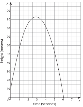
1. How tall is the tower from which the object was shot?
2. When did the object hit the ground?
3. Estimate the greatest height the object reached and the time it took to reach that height. Indicate this situation on the graph.