
5.3.3: Piecewise Linear Functions
- Page ID
- 36033

\( \newcommand{\vecs}[1]{\overset { \scriptstyle \rightharpoonup} {\mathbf{#1}} } \)
\( \newcommand{\vecd}[1]{\overset{-\!-\!\rightharpoonup}{\vphantom{a}\smash {#1}}} \)
\( \newcommand{\id}{\mathrm{id}}\) \( \newcommand{\Span}{\mathrm{span}}\)
( \newcommand{\kernel}{\mathrm{null}\,}\) \( \newcommand{\range}{\mathrm{range}\,}\)
\( \newcommand{\RealPart}{\mathrm{Re}}\) \( \newcommand{\ImaginaryPart}{\mathrm{Im}}\)
\( \newcommand{\Argument}{\mathrm{Arg}}\) \( \newcommand{\norm}[1]{\| #1 \|}\)
\( \newcommand{\inner}[2]{\langle #1, #2 \rangle}\)
\( \newcommand{\Span}{\mathrm{span}}\)
\( \newcommand{\id}{\mathrm{id}}\)
\( \newcommand{\Span}{\mathrm{span}}\)
\( \newcommand{\kernel}{\mathrm{null}\,}\)
\( \newcommand{\range}{\mathrm{range}\,}\)
\( \newcommand{\RealPart}{\mathrm{Re}}\)
\( \newcommand{\ImaginaryPart}{\mathrm{Im}}\)
\( \newcommand{\Argument}{\mathrm{Arg}}\)
\( \newcommand{\norm}[1]{\| #1 \|}\)
\( \newcommand{\inner}[2]{\langle #1, #2 \rangle}\)
\( \newcommand{\Span}{\mathrm{span}}\) \( \newcommand{\AA}{\unicode[.8,0]{x212B}}\)
\( \newcommand{\vectorA}[1]{\vec{#1}} % arrow\)
\( \newcommand{\vectorAt}[1]{\vec{\text{#1}}} % arrow\)
\( \newcommand{\vectorB}[1]{\overset { \scriptstyle \rightharpoonup} {\mathbf{#1}} } \)
\( \newcommand{\vectorC}[1]{\textbf{#1}} \)
\( \newcommand{\vectorD}[1]{\overrightarrow{#1}} \)
\( \newcommand{\vectorDt}[1]{\overrightarrow{\text{#1}}} \)
\( \newcommand{\vectE}[1]{\overset{-\!-\!\rightharpoonup}{\vphantom{a}\smash{\mathbf {#1}}}} \)
\( \newcommand{\vecs}[1]{\overset { \scriptstyle \rightharpoonup} {\mathbf{#1}} } \)
\( \newcommand{\vecd}[1]{\overset{-\!-\!\rightharpoonup}{\vphantom{a}\smash {#1}}} \)
Lesson
Let's explore functions built out of linear pieces.
Exercise \(\PageIndex{1}\): Notice and Wonder: Lines on Dots
What do you notice? What do you wonder?

Exercise \(\PageIndex{2}\): Modeling Recycling
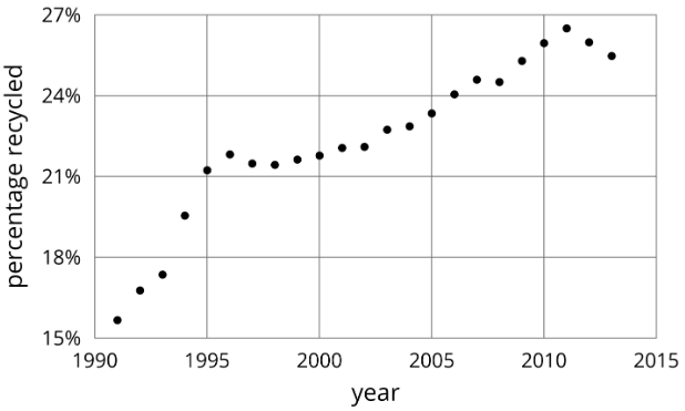
- Approximate the percentage recycled each year with a piecewise linear function by drawing between three and five line segments to approximate the graph.
- Find the slope for each piece. What do these slopes tell you?
Exercise \(\PageIndex{3}\): Dog Bath
Elena filled up the tub and gave her dog a bath. Then she let the water out of the tub.

- The graph shows the amount of water in the tub, in gallons, as a function of time, in minutes. Add labels to the graph to show this.
- When did she turn off the water faucet?
- How much water was in the tub when she bathed her dog?
- How long did it take for the tub to drain completely?
- At what rate did the faucet fill the tub?
- At what rate did the water drain from the tub?
Exercise \(\PageIndex{4}\): Distance and Speed
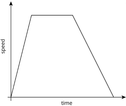
The graph shows the speed of a car as a function of time. Describe what a person watching the car would see.
Are you ready for more?
The graph models the speed of a car over a function of time during a
3-hour trip. How far did the car go over the course of the trip?
There is a nice way to visualize this quantity in terms of the graph. Can you find it?

Summary
This graph shows Andre biking to his friend’s house where he hangs out for a while. Then they bike together to the store to buy some groceries before racing back to Andre’s house for a movie night. Each line segment in the graph represents a different part of Andre’s travels.

This is an example of a piecewise linear function, which is a function whose graph is pieced together out of line segments. It can be used to model situations in which a quantity changes at a constant rate for a while, then switches to a different constant rate.
We can use piecewise functions to represent stories, or we can use them to model actual data. In the second example, temperature recordings at several times throughout a day are modeled with a piecewise function made up of two line segments. Which line segment do you think does the best job of modeling the data?

Practice
Exercise \(\PageIndex{5}\)
The graph shows the distance of a car from home as a function of time.

Describe what a person watching the car may be seeing.
Exercise \(\PageIndex{6}\)
The equation and the graph represent two functions. Use the equation \(y=4\) and the graph to answer the questions.

- When \(x\) is 4, is the output of the equation or the graph greater?
- What value for \(x\) produces the same output in both the graph and the equation?
(From Unit 5.2.5)
Exercise \(\PageIndex{7}\)
This graph shows a trip on a bike trail. The trail has markers every 0.5 km showing the distance from the beginning of the trail.
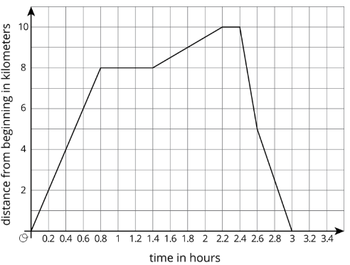
- When was the bike rider going the fastest?
- When was the bike rider going the slowest?
- During what times was the rider going away from the beginning of the trail?
- During what times was the rider going back towards the beginning of the trail?
- During what times did the rider stop?
Exercise \(\PageIndex{8}\)
The expression \(-25t+1250\) represents the volume of liquid of a container after \(t\) seconds. The expression \(50t+250\) represents the volume of liquid of another container after \(t\) seconds. What does the equation \(-25t+1250=50t+250\) mean in this situation?
(From Unit 4.2.8)