
11.3: Graphing Linear Equations (Part 1)
- Page ID
- 5041

\( \newcommand{\vecs}[1]{\overset { \scriptstyle \rightharpoonup} {\mathbf{#1}} } \)
\( \newcommand{\vecd}[1]{\overset{-\!-\!\rightharpoonup}{\vphantom{a}\smash {#1}}} \)
\( \newcommand{\dsum}{\displaystyle\sum\limits} \)
\( \newcommand{\dint}{\displaystyle\int\limits} \)
\( \newcommand{\dlim}{\displaystyle\lim\limits} \)
\( \newcommand{\id}{\mathrm{id}}\) \( \newcommand{\Span}{\mathrm{span}}\)
( \newcommand{\kernel}{\mathrm{null}\,}\) \( \newcommand{\range}{\mathrm{range}\,}\)
\( \newcommand{\RealPart}{\mathrm{Re}}\) \( \newcommand{\ImaginaryPart}{\mathrm{Im}}\)
\( \newcommand{\Argument}{\mathrm{Arg}}\) \( \newcommand{\norm}[1]{\| #1 \|}\)
\( \newcommand{\inner}[2]{\langle #1, #2 \rangle}\)
\( \newcommand{\Span}{\mathrm{span}}\)
\( \newcommand{\id}{\mathrm{id}}\)
\( \newcommand{\Span}{\mathrm{span}}\)
\( \newcommand{\kernel}{\mathrm{null}\,}\)
\( \newcommand{\range}{\mathrm{range}\,}\)
\( \newcommand{\RealPart}{\mathrm{Re}}\)
\( \newcommand{\ImaginaryPart}{\mathrm{Im}}\)
\( \newcommand{\Argument}{\mathrm{Arg}}\)
\( \newcommand{\norm}[1]{\| #1 \|}\)
\( \newcommand{\inner}[2]{\langle #1, #2 \rangle}\)
\( \newcommand{\Span}{\mathrm{span}}\) \( \newcommand{\AA}{\unicode[.8,0]{x212B}}\)
\( \newcommand{\vectorA}[1]{\vec{#1}} % arrow\)
\( \newcommand{\vectorAt}[1]{\vec{\text{#1}}} % arrow\)
\( \newcommand{\vectorB}[1]{\overset { \scriptstyle \rightharpoonup} {\mathbf{#1}} } \)
\( \newcommand{\vectorC}[1]{\textbf{#1}} \)
\( \newcommand{\vectorD}[1]{\overrightarrow{#1}} \)
\( \newcommand{\vectorDt}[1]{\overrightarrow{\text{#1}}} \)
\( \newcommand{\vectE}[1]{\overset{-\!-\!\rightharpoonup}{\vphantom{a}\smash{\mathbf {#1}}}} \)
\( \newcommand{\vecs}[1]{\overset { \scriptstyle \rightharpoonup} {\mathbf{#1}} } \)
\(\newcommand{\longvect}{\overrightarrow}\)
\( \newcommand{\vecd}[1]{\overset{-\!-\!\rightharpoonup}{\vphantom{a}\smash {#1}}} \)
\(\newcommand{\avec}{\mathbf a}\) \(\newcommand{\bvec}{\mathbf b}\) \(\newcommand{\cvec}{\mathbf c}\) \(\newcommand{\dvec}{\mathbf d}\) \(\newcommand{\dtil}{\widetilde{\mathbf d}}\) \(\newcommand{\evec}{\mathbf e}\) \(\newcommand{\fvec}{\mathbf f}\) \(\newcommand{\nvec}{\mathbf n}\) \(\newcommand{\pvec}{\mathbf p}\) \(\newcommand{\qvec}{\mathbf q}\) \(\newcommand{\svec}{\mathbf s}\) \(\newcommand{\tvec}{\mathbf t}\) \(\newcommand{\uvec}{\mathbf u}\) \(\newcommand{\vvec}{\mathbf v}\) \(\newcommand{\wvec}{\mathbf w}\) \(\newcommand{\xvec}{\mathbf x}\) \(\newcommand{\yvec}{\mathbf y}\) \(\newcommand{\zvec}{\mathbf z}\) \(\newcommand{\rvec}{\mathbf r}\) \(\newcommand{\mvec}{\mathbf m}\) \(\newcommand{\zerovec}{\mathbf 0}\) \(\newcommand{\onevec}{\mathbf 1}\) \(\newcommand{\real}{\mathbb R}\) \(\newcommand{\twovec}[2]{\left[\begin{array}{r}#1 \\ #2 \end{array}\right]}\) \(\newcommand{\ctwovec}[2]{\left[\begin{array}{c}#1 \\ #2 \end{array}\right]}\) \(\newcommand{\threevec}[3]{\left[\begin{array}{r}#1 \\ #2 \\ #3 \end{array}\right]}\) \(\newcommand{\cthreevec}[3]{\left[\begin{array}{c}#1 \\ #2 \\ #3 \end{array}\right]}\) \(\newcommand{\fourvec}[4]{\left[\begin{array}{r}#1 \\ #2 \\ #3 \\ #4 \end{array}\right]}\) \(\newcommand{\cfourvec}[4]{\left[\begin{array}{c}#1 \\ #2 \\ #3 \\ #4 \end{array}\right]}\) \(\newcommand{\fivevec}[5]{\left[\begin{array}{r}#1 \\ #2 \\ #3 \\ #4 \\ #5 \\ \end{array}\right]}\) \(\newcommand{\cfivevec}[5]{\left[\begin{array}{c}#1 \\ #2 \\ #3 \\ #4 \\ #5 \\ \end{array}\right]}\) \(\newcommand{\mattwo}[4]{\left[\begin{array}{rr}#1 \amp #2 \\ #3 \amp #4 \\ \end{array}\right]}\) \(\newcommand{\laspan}[1]{\text{Span}\{#1\}}\) \(\newcommand{\bcal}{\cal B}\) \(\newcommand{\ccal}{\cal C}\) \(\newcommand{\scal}{\cal S}\) \(\newcommand{\wcal}{\cal W}\) \(\newcommand{\ecal}{\cal E}\) \(\newcommand{\coords}[2]{\left\{#1\right\}_{#2}}\) \(\newcommand{\gray}[1]{\color{gray}{#1}}\) \(\newcommand{\lgray}[1]{\color{lightgray}{#1}}\) \(\newcommand{\rank}{\operatorname{rank}}\) \(\newcommand{\row}{\text{Row}}\) \(\newcommand{\col}{\text{Col}}\) \(\renewcommand{\row}{\text{Row}}\) \(\newcommand{\nul}{\text{Nul}}\) \(\newcommand{\var}{\text{Var}}\) \(\newcommand{\corr}{\text{corr}}\) \(\newcommand{\len}[1]{\left|#1\right|}\) \(\newcommand{\bbar}{\overline{\bvec}}\) \(\newcommand{\bhat}{\widehat{\bvec}}\) \(\newcommand{\bperp}{\bvec^\perp}\) \(\newcommand{\xhat}{\widehat{\xvec}}\) \(\newcommand{\vhat}{\widehat{\vvec}}\) \(\newcommand{\uhat}{\widehat{\uvec}}\) \(\newcommand{\what}{\widehat{\wvec}}\) \(\newcommand{\Sighat}{\widehat{\Sigma}}\) \(\newcommand{\lt}{<}\) \(\newcommand{\gt}{>}\) \(\newcommand{\amp}{&}\) \(\definecolor{fillinmathshade}{gray}{0.9}\)- Recognize the relation between the solutions of an equation and its graph
- Graph a linear equation by plotting points
- Graph vertical and horizontal lines
Before you get started, take this readiness quiz.
- Evaluate: 3x + 2 when x = −1. If you missed this problem, review Example 3.8.10.
- Solve the formula: 5x + 2y = 20 for y. If you missed this problem, review Example 9.11.6.
- Simplify: \(\dfrac{3}{8}\)(−24). If you missed this problem, review Example 4.3.10.
Recognize the Relation Between the Solutions of an Equation and its Graph
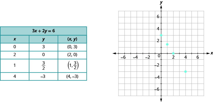
In Use the Rectangular Coordinate System, we found a few solutions to the equation 3x + 2y = 6. They are listed in the table below. So, the ordered pairs (0, 3), (2, 0), \(\left(1, \dfrac{3}{2}\right)\), (4, − 3), are some solutions to the equation 3x + 2y = 6. We can plot these solutions in the rectangular coordinate system as shown on the graph at right.
Notice how the points line up perfectly? We connect the points with a straight line to get the graph of the equation 3x + 2y = 6. Notice the arrows on the ends of each side of the line. These arrows indicate the line continues.
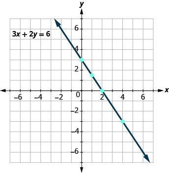
Every point on the line is a solution of the equation. Also, every solution of this equation is a point on this line. Points not on the line are not solutions!
Notice that the point whose coordinates are ( − 2, 6) is on the line shown in Figure \(\PageIndex{1}\). If you substitute x = − 2 and y = 6 into the equation, you find that it is a solution to the equation.
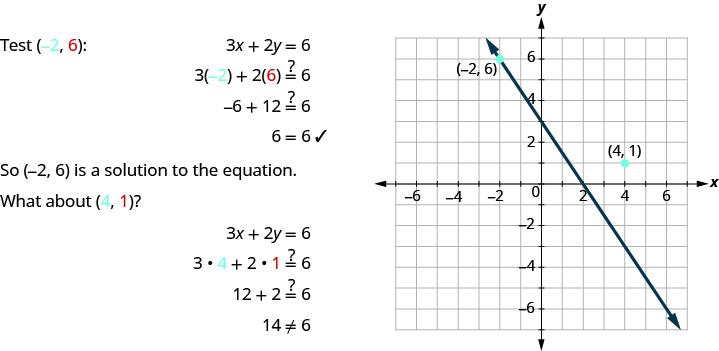
Figure \(\PageIndex{1}\)
So (4, 1) is not a solution to the equation 3x + 2y = 6. Therefore the point (4, 1) is not on the line. This is an example of the saying,” A picture is worth a thousand words.” The line shows you all the solutions to the equation. Every point on the line is a solution of the equation. And, every solution of this equation is on this line. This line is called the graph of the equation 3x + 2y = 6.
The graph of a linear equation Ax + By = C is a straight line.
- Every point on the line is a solution of the equation.
- Every solution of this equation is a point on this line.
The graph of y = 2x − 3 is shown below.
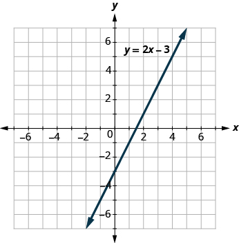
For each ordered pair decide (a) Is the ordered pair a solution to the equation? (b) Is the point on the line?
(a) (0, 3) (b) (3, − 3) (c) (2, − 3) (d) ( − 1, − 5)
Solution
Substitute the x - and y -values into the equation to check if the ordered pair is a solution to the equation.
(a) \[\begin{split} (a)&\; (\textcolor{blue}{0}, \textcolor{red}{-3}) \qquad \qquad \quad \; (b)\; (\textcolor{blue}{3}, \textcolor{red}{3}) \qquad \qquad \qquad \quad (c)\; (\textcolor{blue}{2}, \textcolor{red}{-3}) \qquad \qquad \qquad \quad (d)\; (\textcolor{blue}{-1}, \textcolor{red}{-5}) \\ y &= 2x - 3 \qquad \qquad \quad y = 2x - 3 \qquad \qquad \qquad \; y = 2x - 3 \qquad \qquad \qquad \; \; \; y = 2x - 3 \\ \textcolor{red}{-3} &\stackrel{?}{=} 2(\textcolor{blue}{0}) - 3 \qquad \qquad \; \textcolor{red}{3} \stackrel{?}{=} 2(\textcolor{blue}{3}) - 3 \qquad \qquad \; \textcolor{red}{-3} \stackrel{?}{=} 2(\textcolor{blue}{2}) - 3 \qquad \qquad \; \; \; \textcolor{red}{-5} \stackrel{?}{=} 2(\textcolor{blue}{-1}) - 3 \\ -3 &= -3\; \checkmark \qquad \qquad \quad \; \; 3 = 3\; \checkmark \qquad \qquad \qquad -3 \neq 1 \qquad \qquad \qquad \qquad -5 = -5\; \checkmark \\ (0, -3)\;& is\; a\; solution \ldotp \quad (3, 3)\; is\; a\; solution \ldotp \qquad (2, -3)\; is\; not\; a\; solution \ldotp \qquad (-1, -5)\; is\; a\; solution \ldotp \end{split}\]
(b) Plot the points A: (0, − 3) B: (3, 3) C: (2, − 3) and D: (− 1, − 5). The points (0, − 3), (3, 3), and (− 1, − 5) are on the line y = 2x − 3, and the point (2, − 3) is not on the line.
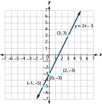
The points which are solutions to y = 2x − 3 are on the line, but the point which is not a solution is not on the line.
The graph of y = 3x − 1 is shown. For each ordered pair, decide (a) is the ordered pair a solution to the equation? (b) is the point on the line?

- (0, − 1)
- (2, 2)
- (3, − 1)
- ( − 1, − 4)
- Answer 1.
-
a. yes, b. no
- Answer 2.
-
a. no, b. no
- Answer 3.
-
a. no, b. no
- Answer 4.
-
a. yes, b. yes
Graph a Linear Equation by Plotting Points
There are several methods that can be used to graph a linear equation. The method we used at the start of this section to graph is called plotting points, or the Point-Plotting Method.
Let’s graph the equation y = 2x + 1 by plotting points. We start by finding three points that are solutions to the equation. We can choose any value for x or y, and then solve for the other variable.
Since y is isolated on the left side of the equation, it is easier to choose values for x. We will use 0, 1, and -2 for x for this example. We substitute each value of x into the equation and solve for y.
We can organize the solutions in a table. See Table \(\PageIndex{1}\).
| y = 2x + 1 | ||
|---|---|---|
| x | y | (x, y) |
| 0 | 1 | (0, 1) |
| 1 | 3 | (1, 3) |
| -2 | -3 | (-2, -3) |
Now we plot the points on a rectangular coordinate system. Check that the points line up. If they did not line up, it would mean we made a mistake and should double-check all our work. See Figure \(\PageIndex{2}\).
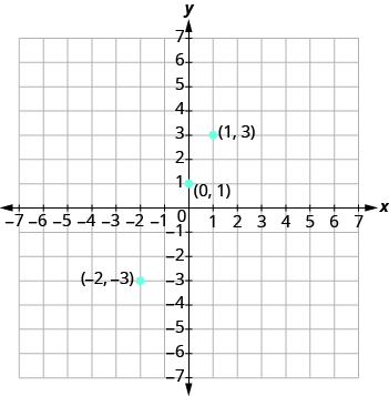
Figure \(\PageIndex{2}\)
Draw the line through the three points. Extend the line to fill the grid and put arrows on both ends of the line. The line is the graph of y = 2x + 1.
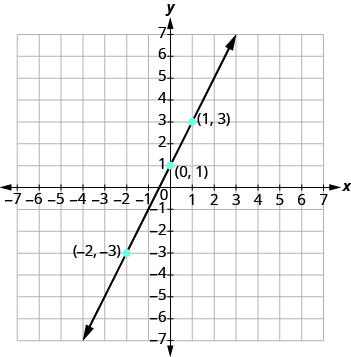
Figure \(\PageIndex{3}\)
Step 1. Find three points whose coordinates are solutions to the equation. Organize them in a table.
Step 2. Plot the points on a rectangular coordinate system. Check that the points line up. If they do not, carefully check your work.
Step 3. Draw the line through the points. Extend the line to fill the grid and put arrows on both ends of the line.
It is true that it only takes two points to determine a line, but it is a good habit to use three points. If you plot only two points and one of them is incorrect, you can still draw a line but it will not represent the solutions to the equation. It will be the wrong line. If you use three points, and one is incorrect, the points will not line up. This tells you something is wrong and you need to check your work. See Figure \(\PageIndex{4}\).
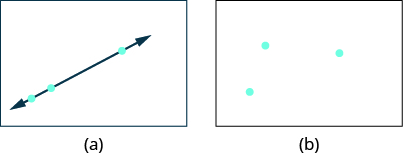
Figure \(\PageIndex{4}\) - Look at the difference between (a) and (b). All three points in (a) line up so we can draw one line through them. The three points in (b) do not line up. We cannot draw a single straight line through all three points.
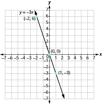
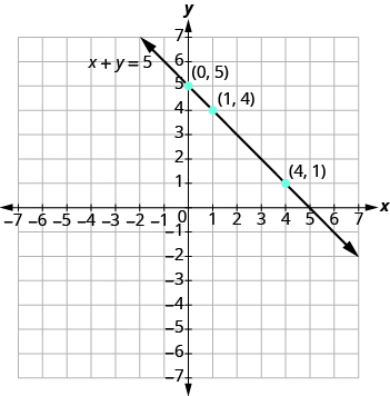
Graph the equation y = −3x.
Solution
Find three points that are solutions to the equation. It’s easier to choose values for x, and solve for y. Do you see why?
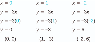
List the points in a table.
| y = −3x | ||
|---|---|---|
| x | y | (x, y) |
| 0 | 0 | (0, 0) |
| 1 | -3 | (1, -3) |
| -2 | 6 | (-2, 6) |
Plot the points, check that they line up, and draw the line as shown.
Graph the equation by plotting points: y = −4x.
- Answer
Graph the equation by plotting points: y = x.
- Answer
-
When an equation includes a fraction as the coefficient of x, we can substitute any numbers for x. But the math is easier if we make ‘good’ choices for the values of x. This way we will avoid fraction answers, which are hard to graph precisely.
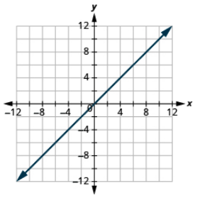
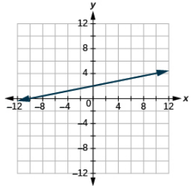
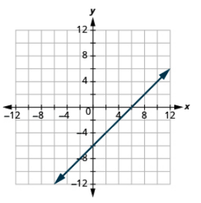
Graph the equation y = \(\dfrac{1}{2}\)x + 3.
Solution
Find three points that are solutions to the equation. Since this equation has the fraction \(\dfrac{1}{2}\) as a coefficient of x, we will choose values of x carefully. We will use zero as one choice and multiples of 2 for the other choices.
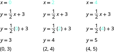
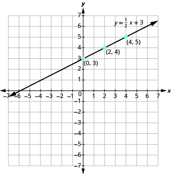
The points are shown in the table.
| y = \(\dfrac{1}{2}\)x + 3 | ||
|---|---|---|
| x | y | (x, y) |
| 0 | 3 | (0, 3) |
| 2 | 4 | (2, 4) |
| 4 | 5 | (4, 5) |
Plot the points, check that they line up, and draw the line as shown.
Graph the equation: y = \(\dfrac{1}{3}\)x − 1
- Answer
-
Graph the equation: y = \(\dfrac{1}{4}\)x + 2.
- Answer
-
So far, all the equations we graphed had y given in terms of x. Now we’ll graph an equation with x and y on the same side.
Graph the equation x + y = 5.
Solution
Find three points that are solutions to the equation. Remember, you can start with any value of x or y.
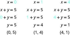
We list the points in a table.
| x + y = 5 | ||
|---|---|---|
| x | y | (x, y) |
| 0 | 5 | (0, 5) |
| 1 | 4 | (1, 4) |
| 4 | 1 | (4, 1) |
Then plot the points, check that they line up, and draw the line.
Graph the equation: x + y = −2.
- Answer
-
Graph the equation: x − y = 6.
- Answer
-
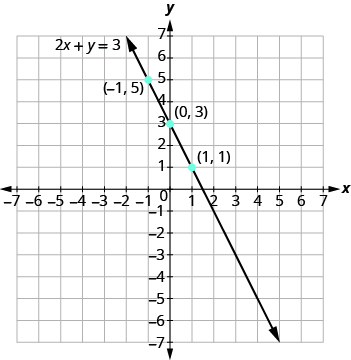
In the previous example, the three points we found were easy to graph. But this is not always the case. Let’s see what happens in the equation 2x + y = 3. If y is 0, what is the value of x?
\[\begin{split} 2x + y &= 3 \\ 2x + \textcolor{red}{0} &= 3 \\ 2x &= 3 \\ x &= \dfrac{3}{2} \end{split}\]
The solution is the point \(\left(\dfrac{3}{2}, 0\right)\). This point has a fraction for the x -coordinate. While we could graph this point, it is hard to be precise graphing fractions. Remember in the example y = \(\dfrac{1}{2}\)x + 3, we carefully chose values for x so as not to graph fractions at all. If we solve the equation 2x + y = 3 for y, it will be easier to find three solutions to the equation.
\[\begin{split} 2x + y &= 3 \\ y &= -2x + 3 \end{split}\]
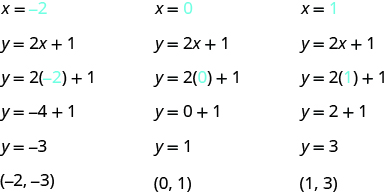
Now we can choose values for x that will give coordinates that are integers. The solutions for x = 0, x = 1, and x = −1 are shown.
| y = −2x + 3 | ||
|---|---|---|
| x | y | (x, y) |
| 0 | 3 | (0, 3) |
| 1 | 1 | (1, 1) |
| -1 | 5 | (-1, 5) |
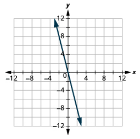
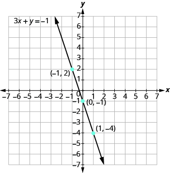
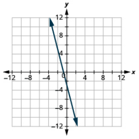
Graph the equation 3x + y = −1.
Solution
Find three points that are solutions to the equation.
First, solve the equation for y.
\[\begin{split} 3x + y &= −1 \\ y &= −3x − 1 \end{split}\]
We’ll let x be 0, 1, and −1 to find three points. The ordered pairs are shown in the table. Plot the points, check that they line up, and draw the line.
| y = −3x − 1 | ||
|---|---|---|
| x | y | (x, y) |
| 0 | -1 | (0, -1) |
| 1 | -4 | (1, -4) |
| -1 | 2 | (-1, 2) |
If you can choose any three points to graph a line, how will you know if your graph matches the one shown in the answers in the book? If the points where the graphs cross the x- and y -axes are the same, the graphs match.
Graph each equation: 2x + y = 2.
- Answer
Graph each equation: 4x + y = −3.
- Answer
-
Contributors and Attributions
Lynn Marecek (Santa Ana College) and MaryAnne Anthony-Smith (Formerly of Santa Ana College). This content is licensed under Creative Commons Attribution License v4.0 "Download for free at http://cnx.org/contents/fd53eae1-fa2...49835c3c@5.191."