2.4: Graphs of the Other Trigonometric Functions

Focus Questions

The following questions are meant to guide our study of the material in this section. After studying this section, we should understand the concepts motivated by these questions and be able to write precise, coherent answers to these questions.

• What are the important properties of the graph of \(y = \tan(t)\). That is, what is the domain and what is the range of the tangent function, and what happens to the values of the tangent function at the points that are near points not in the domain of the tangent function?
• What are the important properties of the graph of \(y = \sec(t)\). That is, what is the domain and what is the range of the secant function, and what happens to the values of the secant function at the points that are near points not in the domain of the secant function?
• What are the important properties of the graph of \(y = \cot(t)\). That is, what is the domain and what is the range of the cotangent function, and what happens to the values of the cotangent function at the points that are near points not in the domain of the cotangent function?
• What are the important properties of the graph of \(y = \csc(t)\). That is, what is the domain and what is the range of the cosecant function, and what happens to the values of the cosecant function at the points that are near points not in the domain of the cosecant function?

We have seen how the graphs of the cosine and sine functions are determined by the definition of these functions. We also investigated the effects of the constants \(A, B, C\), and \(D\) on the graph of \(y = A\sin(B(x - C)) + D\) and the graph of \(y = A\sin(B(x - C)) + D\).

In the following beginning activity, we will explore the graph of the tangent function. Later in this section, we will discuss the graph of the secant function, and the graphs of the cotangent and cosecant functions will be explored in the exercises. One of the key features of these graphs is the fact that they all have vertical asymptotes. Important information about all four functions is summarized at the end of this section.

Beginning Activity

1. Use a graphing utility to draw the graph of \(f(x) = \dfrac{1}{(x+1)(x-1)}\) using \(-2 \leq x \leq 2\) and \(-10 \leq y \leq 10\). If possible, use the graphing utility to draw the graphs of the vertical lines \(x = -1\) and \(x = 1\). The graph of the function \(f\) has vertical asymptotes \(x = -1\) and \(x = 1\). The reason for this is that at these values of \(x\), the numerator of the function is not zero and the denominator is 0. So \(x = -1\) and \(x = 1\) are not in the domain of this function. In general, if a function is a quotient of two functions, then there will be a vertical asymptote for those values of x for which the numerator is not zero and the denominator is zero. We will see this for the the tangent, cotangent, secant, and cosecant functions.
2. How is the tangent function defined? Complete the following: For each real number \(x\) with \(\cos(t) \neq 0, \tan(t) = ?\).
3. Use a graphing utility to draw the graph of \(y = \tan(t)\) using \(-\pi \leq t \leq \pi\) and \(-10 \leq y \leq 10\).
4. What are some of the vertical asymptotes of the graph of the function \(y = \tan(t)\)? What appears to be the range of the tangent function?

The Graph of the Tangent Function

The graph of the tangent function is very different than the graphs of the sine and cosine functions. One reason is that because \(\tan(t) = \dfrac{\sin(t)}{\cos(t)}\), there are values of \(t\) for which \(\tan(t)\) is not defined. We have seen that the domain of the tangent function is the set of all real numbers \(t\) for which \(t = \neq \dfrac{\pi}{2} + k\pi\) for every integer \(k\).

In particular, the real numbers \(\dfrac{\pi}{2}\) and \(-\dfrac{\pi}{2}\) are not in the domain of the tangent function. So the graph of the tangent function will have vertical asymptotes at \(t = \dfrac{\pi}{2}\) and \(t = -\dfrac{\pi}{2}\) (as well as at other values). We should have observed this in the beginning activity.

So to draw an accurate graph of the tangent function, it will be necessary to understand the behavior of the tangent near the points that are not in its domain. We now investigate the behavior of the tangent for points whose values of \(t\) that are slightly less than \(\dfrac{\pi}{2}\) and for points whose values of t that are slightly greater than \(-\dfrac{\pi}{2}\). Using a calculator, we can obtain the values shown in Table 2.4.

\(t\)	\(\tan(t)\)
\(\dfrac{\pi}{2} - 0.1\)	9.966644423
\(\dfrac{\pi}{2} - 0.01\)	99.99666664
\(\dfrac{\pi}{2} - 0.001\)	999.9996667
\(\dfrac{\pi}{2} - 0.0001\)	9999.999967
\(\dfrac{\pi}{2} + 0.1\)	-9.966644423
\(\dfrac{\pi}{2} + 0.01\)	-99.99666664
\(\dfrac{\pi}{2} + 0.001\)	-999.9996667
\(\dfrac{\pi}{2} + 0.0001\)	-9999.999967

Table 2.4: Table of Values for the Tangent Function

So as the input \(t\) gets close to \(\dfrac{\pi}{2}\) but stays less than \(\dfrac{\pi}{2}\), the values of \(\tan(t)\) are getting larger and larger, seemingly without bound. Similarly, input \(t\) gets close to \(-\dfrac{\pi}{2}\) but stays greater than \(-\dfrac{\pi}{2}\), the values of tan.t / are getting farther and farther away from 0 in the negative direction, seemingly without bound. We can see this in the definition of the tangent: as \(t\) gets close to \(\dfrac{\pi}{2}\) from the left, \(\cos(t)\) gets close to 0 and \(\sin(t)\) gets close to 1. Now \(\tan(t) = \dfrac{\sin(t)}{\cos(t)}\) and fractions where the numerator is close to \(1\) and the denominator close to \(0\) have very large values. Similarly, as t gets close to \(-\dfrac{\pi}{2}\) from the right, \(\cos(t)\) gets close to \(0\) (but is negative) and \(\sin(t)\) gets close to \(1\). Fractions where the numerator is close to 1 and the denominator close to 0, but negative, are very large (in magnitude) negative numbers.

Exercise \(\PageIndex{1}\)

1. Use a graphing utility to draw the graph of \(y = \tan(t)\) using \(-\dfrac{\pi}{2} \leq t \leq \dfrac{\pi}{2}\) and \(-10 \leq y \leq 10\).
2. Use a graphing utility to draw the graph of \(y = \tan(t)\) using \(-\dfrac{3\pi}{2} \leq t \leq \dfrac{3\pi}{2}\) and \(-10 \leq y \leq 10\).
3. Are these graphs consistent with the information we have discussed about vertical asymptotes for the tangent function?
4. What appears to be the range of the tangent function?
5. What appears to be the period of the tangent function?

Answer

The graphs for (1) and (2) are shown below.

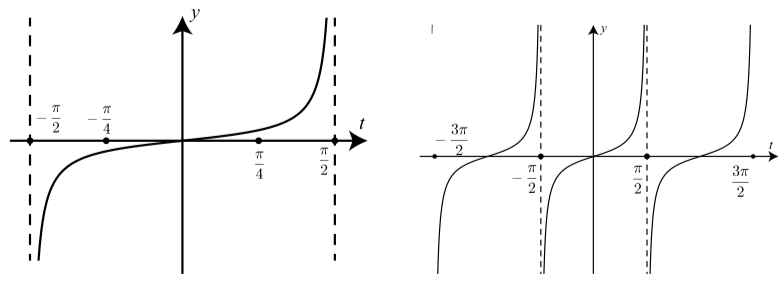
In both graphs, the graph just to the left of \(t = \dfrac{\pi}{2}\) and just to the right of \(t = -\dfrac{\pi}{2}\) is consistent with the information in Table 2.4. The graph on the

right is also consistent with the information in this table on both sides of \(t = \dfrac{\pi}{2}\) and \(t = -\dfrac{\pi}{2}\)

The range of the tangent function is the set of all real numbers.

Based on the graph in(2), the period of the tangent function appears to be \(\pi\). The period is actually equal to \(\pi\), and more information about this is given in Exercise (1).

Activity 2.22 (The Tangent Function and the Unit Circle)

The diagram in Figure \(\PageIndex{1}\) can be used to show how \(\tan(t)\) is related to the unit circle definitions of \(\cos(t)\) and \(\sin(t)\).

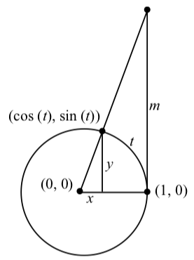
Figure \(\PageIndex{1}\): Illustrating \(\tan(t)\) with the Unit Circle

In the diagram, an arc of length t is drawn and \(\tan(t) = \dfrac{\cos(t)}{\sin(t)} = \dfrac{y}{x}\). This gives the slope of the line that goes through the points \((0, 0)\) and \((\cos(t), \sin(t))\). The vertical line through the point \((1, 0)\) intersects this line at the point \((1, m)\). This means that the slope of this line is also m and hence, we see that \[\tan(t) = \dfrac{\cos(t)}{\sin(t)} = m.\]

Now use the Geogebra applet Tangent Graph Generator to see how this information can be used to help see how the graph of the tangent function can be generated using the ideas in Figure \(\PageIndex{1}\). The web address is http://gvsu.edu/s/Zm

Effects of Constants on the Graphs of the Tangent Function

There are similarities and a some differences in the methods of drawing the graph of a function of the form \(y = A\tan(B(t - C)) + D\) and drawing the graph of a function of the form \(y = A\sin(B(t - C)) + D\). See page 101 for a summary of the effects of the parameters \(A, B, C\), and \(D\) on the graph of a sinusoidal function.

One of the differences in dealing with a tangent (secant, cotangent, or cosecant) function is that we do not use the terminology that is specific to sinusoidal waves. In particular, we will not use the terms amplitude and phase shift. Instead of amplitude, we use the more general term vertical stretch (or vertical compression), and instead of phase shift, we use the more general term horizontal shift. We will explore this is the following progress check.

Exercise \(\PageIndex{2}\)

Consider the function whose equation is \(y = 3\tan(2(x - \dfrac{\pi}{8})) + 1\). Even if we use a graphing utility to draw the graph, we should answer the following questions first in order to get a reasonable viewing window for the graphing utility. It might be a good idea to use a method similar to what we would use if we were graphing \(y = 3\sin(2(x - \dfrac{\pi}{8})) + 1\)

1. We know that for the sinusoid, the period is \(\dfrac{2\pi}{2}\). However, the period of the tangent function is \(\pi\). So what will be the period of \(y = 3\tan(2(x - \dfrac{\pi}{8})) + 1\)?
2. For the sinusoid, the amplitude is 3. However, we do not use the term “amplitude” for the tangent. So what is the effect of the parameter 2 on the graph of \(y = 3\tan(2(x - \dfrac{\pi}{8})) + 1\)?
3. For the sinusoid, the phase shift is \(\dfrac{\pi}{8}\). However, we do not use the term “phase shift” for the tangent. So what is the effect of the parameter 8 on the graph of \(y = 3\tan(2(x - \dfrac{\pi}{8})) + 1\)?
4. Use a graphing utility to draw the graph of this function for one complete period. Use the period of the function that contains the number 0.

Answer

1. The equation for the function is \(y = 3\tan(2(x - \dfrac{\pi}{8})) + 1\)
2. The period of this function is \(\dfrac{\pi}{2}\).
3. The effect of the parameter \(3\) is to vertically stretch the graph of the tangent function.
4. Following is a graph of one period of this function using \(-\dfrac{\pi}{8} \leq x \leq \dfrac{3\pi}{8}\) and \(-20 \leq y \leq 20\). The vertical asymptotes at \(x = -\dfrac{\pi}{8}\) \(x = \dfrac{3\pi}{8}\) are shown as well as the horizontal line \(y = 1\).

• The effect of the parameter \(\dfrac{\pi}{8}\) is to shift the graph of \(y = 3\tan(2(x)) + 1\) to the right by \(\dfrac{\pi}{8}\) units.

The Graph of the Secant Function

To understand the graph of the secant function, we need to recall the definition of the secant and the restrictions on its domain. If necessary, refer to Section 1.6 to complete the following progress check.

Exercise \(\PageIndex{3}\)

1. How is the secant function defined?
2. What is the domain of the secant function?
3. Where will the graph of the secant function have vertical asymptotes?
4. What is the period of the secant function?

Answer

The secant function is the reciprocal of the cosine function. That is, \(\sec(t) = \dfrac{1}{\cos(t)}\)

The domain of the secant function is the set of all real numbers \(t\) for which \(t \neq \dfrac{\pi}{2} + k\pi\) for every integer \(k\).

The graph of the secant function will have a vertical asymptote at those values of \(t\) that are not in the domain. So there will be a vertical asymptote when \(t = \dfrac{\pi}{2} + k\pi\) for some integer \(k\).

Since \(\sec(t) = \dfrac{1}{\cos(t)}\), and the period of the cosine function is \(2\pi\), we conclude that the period of the secant function is also \(2\pi\).

Activity 2.25 (The Graph of the Secant Function)

We will use the Geogebra Applet with the following web address: http://gvsu.edu/s/Zn This applet will show how the graph of the secant function is related to the graph of the cosine function. In the applet, the graph of \(y = \cos(t)\) is shown and is left fixed. We generate points on the graph of \(y = \sec(t)\) by using the slider for t. For each value of \(t\), a vertical line is drawn from the point \((t, \cos(t))\) to the point \((t, \sec(t))\). Notice how these points indicate that the graph of the secant function has vertical asymptotes at \(t = \dfrac{\pi}{2}, t = \dfrac{3\pi}{2}\) and \(\dfrac{5\pi}{2}\).

• Use a graphing utility to draw the graph of \(y = \sec(t)\) using \(-\dfrac{\pi}{2} \leq x \leq \dfrac{\pi}{2}\) and \(-10 \leq y \leq 10\). Note: It may be necessary to use \(\sec(x) = \dfrac{1}{\cos(x)}\)
• Use a graphing utility to draw the graph of \(y = \sec(t)\) using \(-\dfrac{3\pi}{2} \leq x \leq \dfrac{3\pi}{2}\) and \(-10 \leq y \leq 10\).
• The work in Activity 2.25 and Figure \(\PageIndex{2}\) can be used to help answer the questions in Exercise \(\PageIndex{3}\).

  

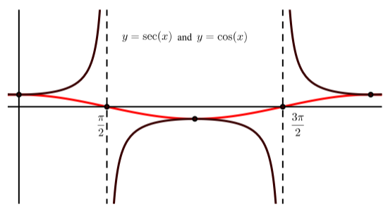
  Figure \(\PageIndex{2}\): Graph of One Period of \(y = \sec(t)\) with \(0 \ leq x \ leq 2\pi\)

Exercise \(\PageIndex{4}\)

1. Is the graph in Figure \(\PageIndex{2}\) consistent with the graphs from Activity 2.25?
2. Why is the graph of \(y = \sec(t)\) above the x-axis when \(-\dfrac{\pi}{2} \leq x \leq \dfrac{\pi}{2}\)?
3. Why is the graph of \(y = \sec(t)\) below the x-axis when \(\dfrac{\pi}{2} \leq x \leq \dfrac{3\pi}{2}\)
4. What is the range of the secant function?

Answer

All of the graphs are consistent.

Since \(\sec(x) = \dfrac{1}{\cos(x)}\), we see that \(\sec(x) > 0\) if and only if \(\cos(x) > 0\). So the graph of \(y = \sec(x)\) is above the \(x\)-axis if and only if the graph of \(y = \cos(x)\) is above the \(x\)-axis.

3. Since \(\sec(x) = \dfrac{1}{\cos(x)}\), we see that \(\sec(x) < 0\) if and only if \(\cos(x) < 0\). So the graph of \(y = \sec(x)\) is below the \(x\)-axis if and only if the graph of \(y = \cos(x)\) is above the \(x\)-axis.

The key is that \(\sec(x) = \dfrac{1}{\cos(x)}\). Since \(-1 \leq \cos(x) \leq 1\), we conclude that \(\sec(x) \geq 1\) when \(\cos(x) > 0\) and \(\sec(x) \leq -1\) when \(\cos(x) < 0\). Since the graph of the secant function has vertical asymptotes, we see that the range of the secant function consists of all real numbers \(y\) for which \(y \geq 1\) or \(y \leq -1\). This can also be seen on the graph of \(y = \sec(x)\).

Summary

In this section, we studied the following important concepts and ideas:

The Tangent Function. Table 2.5 shows some of the important characteristics of the tangent function. We have already discussed most of these items, but the last two items in this table will be explored in Exercise (1) and Exercise (2). A graph of three periods of the tangent function is shown in Figure \(\PageIndex{3}\).

	\(y = \tan(t)\)	\(y = \sec(t)\)
period	\(\pi\)	\(2\pi\)
domain	real numbers \(t\) with \(t \neq \dfrac{\pi}{2}+k\pi\) for every integer \(k\)	real numbers \(t\) with \(t \neq \dfrac{\pi}{2}+k\pi\) for every integer \(k\)
\(y\)-intercept	\((0, 0)\)	\((0, 1)\)
\(x\)-intercepts	\(t = k\pi\), where \(k\) is some integer	none
symmetry	with respect to the origin	with respect to the \(y\)-axis

Table 2.5: Properties of the Tangent and Secant Functions

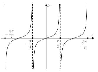
Figure \(\PageIndex{3}\): Graph of \(y = \tan(t)\)

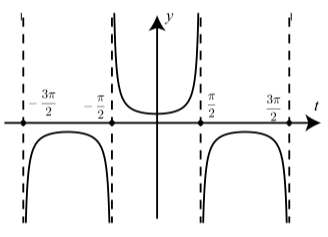
Figure \(\PageIndex{4}\): Graph of \(y = \sec(t)\)

The Secant Function. Table 2.5 shows some of the important characteristics of the secant function. The symmetry of the secant function is explored in Exercise (3). Figure 2.29 shows a graph of the secant function.

The Cosecant Function. The graph of the cosecant function is studied in a way that is similar to how we studied the graph of the secant function. This is done in Exercises (4), (5), and (6). Table 2.6 shows some of the important characteristics of the cosecant function. The symmetry of the cosecant function is explored in Exercise (3). Figure 2.30 shows a graph of the cosecant function.

The Cotangent Function. The graph of the cosecant function is studied in a way that is similar to how we studied the graph of the tangent function. This is done in Exercises (7), (8), and (9). Table 2.6 shows some of the important characteristics of the cotangent function. The symmetry of the cotangent function is explored in Exercise (3). Figure 2.31 shows a graph of the cotangent function.

	\(y = \csc(t)\)	\(y = \cot(t)\)
period	\(2\pi\)	\(\pi\)
domain	real numbers \(t\) with \(t \neq k\pi\) for every integer \(k\)	real numbers \(t\) with \(t \neq k\pi\) for every integer \(k\)
range	\(|y| \geq 1\)	all real numbers
\(y\)-intercept	none	none
\(x\)-intercepts	none	\(t = \dfrac{\pi}{2}+k\pi\) where \(k\) is an integer
symmetry	with respect to the origin	with respect to the origin

Table 2.6: Properties of the Cosecant and Cotangent Functions

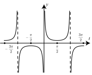
Figure \(\PageIndex{5}\): Graph of \(y = \csc(t)\)

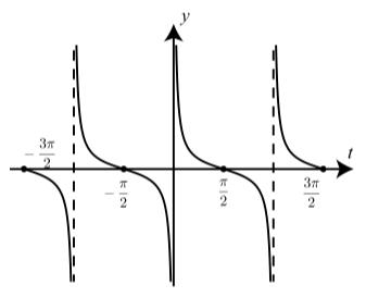
Figure \(\PageIndex{6}\): Graph of \(y = \cot(t)\)