
2.1: Linear Functions
- Page ID
- 3982
\( \newcommand{\vecs}[1]{\overset { \scriptstyle \rightharpoonup} {\mathbf{#1}} } \)
\( \newcommand{\vecd}[1]{\overset{-\!-\!\rightharpoonup}{\vphantom{a}\smash {#1}}} \)
\( \newcommand{\dsum}{\displaystyle\sum\limits} \)
\( \newcommand{\dint}{\displaystyle\int\limits} \)
\( \newcommand{\dlim}{\displaystyle\lim\limits} \)
\( \newcommand{\id}{\mathrm{id}}\) \( \newcommand{\Span}{\mathrm{span}}\)
( \newcommand{\kernel}{\mathrm{null}\,}\) \( \newcommand{\range}{\mathrm{range}\,}\)
\( \newcommand{\RealPart}{\mathrm{Re}}\) \( \newcommand{\ImaginaryPart}{\mathrm{Im}}\)
\( \newcommand{\Argument}{\mathrm{Arg}}\) \( \newcommand{\norm}[1]{\| #1 \|}\)
\( \newcommand{\inner}[2]{\langle #1, #2 \rangle}\)
\( \newcommand{\Span}{\mathrm{span}}\)
\( \newcommand{\id}{\mathrm{id}}\)
\( \newcommand{\Span}{\mathrm{span}}\)
\( \newcommand{\kernel}{\mathrm{null}\,}\)
\( \newcommand{\range}{\mathrm{range}\,}\)
\( \newcommand{\RealPart}{\mathrm{Re}}\)
\( \newcommand{\ImaginaryPart}{\mathrm{Im}}\)
\( \newcommand{\Argument}{\mathrm{Arg}}\)
\( \newcommand{\norm}[1]{\| #1 \|}\)
\( \newcommand{\inner}[2]{\langle #1, #2 \rangle}\)
\( \newcommand{\Span}{\mathrm{span}}\) \( \newcommand{\AA}{\unicode[.8,0]{x212B}}\)
\( \newcommand{\vectorA}[1]{\vec{#1}} % arrow\)
\( \newcommand{\vectorAt}[1]{\vec{\text{#1}}} % arrow\)
\( \newcommand{\vectorB}[1]{\overset { \scriptstyle \rightharpoonup} {\mathbf{#1}} } \)
\( \newcommand{\vectorC}[1]{\textbf{#1}} \)
\( \newcommand{\vectorD}[1]{\overrightarrow{#1}} \)
\( \newcommand{\vectorDt}[1]{\overrightarrow{\text{#1}}} \)
\( \newcommand{\vectE}[1]{\overset{-\!-\!\rightharpoonup}{\vphantom{a}\smash{\mathbf {#1}}}} \)
\( \newcommand{\vecs}[1]{\overset { \scriptstyle \rightharpoonup} {\mathbf{#1}} } \)
\(\newcommand{\longvect}{\overrightarrow}\)
\( \newcommand{\vecd}[1]{\overset{-\!-\!\rightharpoonup}{\vphantom{a}\smash {#1}}} \)
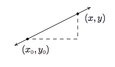
\(\newcommand{\avec}{\mathbf a}\) \(\newcommand{\bvec}{\mathbf b}\) \(\newcommand{\cvec}{\mathbf c}\) \(\newcommand{\dvec}{\mathbf d}\) \(\newcommand{\dtil}{\widetilde{\mathbf d}}\) \(\newcommand{\evec}{\mathbf e}\) \(\newcommand{\fvec}{\mathbf f}\) \(\newcommand{\nvec}{\mathbf n}\) \(\newcommand{\pvec}{\mathbf p}\) \(\newcommand{\qvec}{\mathbf q}\) \(\newcommand{\svec}{\mathbf s}\) \(\newcommand{\tvec}{\mathbf t}\) \(\newcommand{\uvec}{\mathbf u}\) \(\newcommand{\vvec}{\mathbf v}\) \(\newcommand{\wvec}{\mathbf w}\) \(\newcommand{\xvec}{\mathbf x}\) \(\newcommand{\yvec}{\mathbf y}\) \(\newcommand{\zvec}{\mathbf z}\) \(\newcommand{\rvec}{\mathbf r}\) \(\newcommand{\mvec}{\mathbf m}\) \(\newcommand{\zerovec}{\mathbf 0}\) \(\newcommand{\onevec}{\mathbf 1}\) \(\newcommand{\real}{\mathbb R}\) \(\newcommand{\twovec}[2]{\left[\begin{array}{r}#1 \\ #2 \end{array}\right]}\) \(\newcommand{\ctwovec}[2]{\left[\begin{array}{c}#1 \\ #2 \end{array}\right]}\) \(\newcommand{\threevec}[3]{\left[\begin{array}{r}#1 \\ #2 \\ #3 \end{array}\right]}\) \(\newcommand{\cthreevec}[3]{\left[\begin{array}{c}#1 \\ #2 \\ #3 \end{array}\right]}\) \(\newcommand{\fourvec}[4]{\left[\begin{array}{r}#1 \\ #2 \\ #3 \\ #4 \end{array}\right]}\) \(\newcommand{\cfourvec}[4]{\left[\begin{array}{c}#1 \\ #2 \\ #3 \\ #4 \end{array}\right]}\) \(\newcommand{\fivevec}[5]{\left[\begin{array}{r}#1 \\ #2 \\ #3 \\ #4 \\ #5 \\ \end{array}\right]}\) \(\newcommand{\cfivevec}[5]{\left[\begin{array}{c}#1 \\ #2 \\ #3 \\ #4 \\ #5 \\ \end{array}\right]}\) \(\newcommand{\mattwo}[4]{\left[\begin{array}{rr}#1 \amp #2 \\ #3 \amp #4 \\ \end{array}\right]}\) \(\newcommand{\laspan}[1]{\text{Span}\{#1\}}\) \(\newcommand{\bcal}{\cal B}\) \(\newcommand{\ccal}{\cal C}\) \(\newcommand{\scal}{\cal S}\) \(\newcommand{\wcal}{\cal W}\) \(\newcommand{\ecal}{\cal E}\) \(\newcommand{\coords}[2]{\left\{#1\right\}_{#2}}\) \(\newcommand{\gray}[1]{\color{gray}{#1}}\) \(\newcommand{\lgray}[1]{\color{lightgray}{#1}}\) \(\newcommand{\rank}{\operatorname{rank}}\) \(\newcommand{\row}{\text{Row}}\) \(\newcommand{\col}{\text{Col}}\) \(\renewcommand{\row}{\text{Row}}\) \(\newcommand{\nul}{\text{Nul}}\) \(\newcommand{\var}{\text{Var}}\) \(\newcommand{\corr}{\text{corr}}\) \(\newcommand{\len}[1]{\left|#1\right|}\) \(\newcommand{\bbar}{\overline{\bvec}}\) \(\newcommand{\bhat}{\widehat{\bvec}}\) \(\newcommand{\bperp}{\bvec^\perp}\) \(\newcommand{\xhat}{\widehat{\xvec}}\) \(\newcommand{\vhat}{\widehat{\vvec}}\) \(\newcommand{\uhat}{\widehat{\uvec}}\) \(\newcommand{\what}{\widehat{\wvec}}\) \(\newcommand{\Sighat}{\widehat{\Sigma}}\) \(\newcommand{\lt}{<}\) \(\newcommand{\gt}{>}\) \(\newcommand{\amp}{&}\) \(\definecolor{fillinmathshade}{gray}{0.9}\)We now begin the study of families of functions. Our first family, linear functions, are old friends as we shall soon see. Recall from Geometry that two distinct points in the plane determine a unique line containing those points, as indicated below.
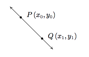
To give a sense of the 'steepness' of the line, we recall that we can compute the slope of the line using the formula below.
The slope \(m\) of the line containing the points \(P\left(x_0, y_0\right)\) and \(Q\left(x_1, y_1\right)\) is:
\[ m = \dfrac{y_{1} - y_0}{x_{1} - x_0},\label{slope} \]
provided \(x_1 \neq x_0\).
A couple of notes about Equation 2.1 are in order. First, don't ask why we use the letter '\(m\)' to represent slope. There are many explanations out there, but apparently no one really knows for sure. Secondly, the stipulation \(x_{1 \neq x_0}\) ensures that we aren't trying to divide by zero. The reader is invited to pause to think about what is happening geometrically; the anxious reader can skip along to the next example.
Example \(\PageIndex{1}\):
Find the slope of the line containing the following pairs of points, if it exists. Plot each pair of points and the line containing them.
- \(P(0,0)\), \(Q(2,4)\)
- \(P(-1,2)\), \(Q(3,4)\)
- \(P(-2,3)\), \(Q(2,-3)\)
- \(P(-3,2)\), \(Q(4,2)\)
- \(P(2,3)\), \(Q(2,-1)\)
- \(P(2,3)\), \(Q(2.1, -1)\)
Solution
In each of these examples, we apply the slope formula, Equation 2.1.
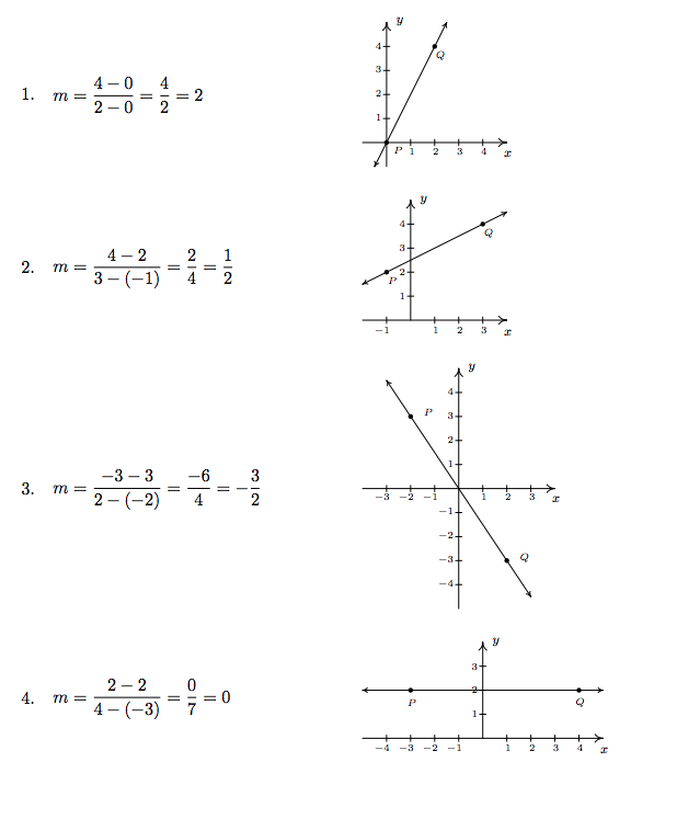
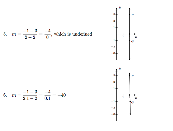
A few comments about Example \(\PageIndex{1}\) are in order. First, for reasons which will be made clear soon, if the slope is positive then the resulting line is said to be increasing. If it is negative, we say the line is decreasing. A slope of \(0\) results in a horizontal line which we say is constant, and an undefined slope results in a vertical line. Some authors use the unfortunate moniker 'no slope' when a slope is undefined. It's easy to confuse the notions of 'no slope' with 'slope of \(0\)'. For this reason, we will describe slopes of vertical lines as 'undefined'. Second, the larger the slope is in absolute value, the steeper the line. You may recall from Intermediate Algebra that slope can be described as the ratio
\[m = \dfrac{\text{ rise}}{\text{ run}}\]
For example, in the second part of Example \(\PageIndex{1}\), we found the slope to be \(\frac{1}{2}\). We can interpret this as a rise of 1 unit upward for every \(2\) units to the right we travel along the line, as shown below.
Using more formal notation, given points \(\left(x_{0}, y_0\right)\) and \(\left(x_1, y_1\right)\), we use the Greek letter delta '\(\Delta\)' to write \(\Delta y = y_1 - y_0\) and \(\Delta x = x_1 - x_0\). In most scientific circles, the symbol \(\Delta\) means 'change in'.
Hence, we may write
\[ m = \dfrac{\Delta y}{\Delta x},\]
which describes the slope as the rate of change of \(y\) with respect to \(x\). Rates of change abound in the 'real world', as the next example illustrates.
Example \(\PageIndex{2}\):
Suppose that two separate temperature readings were taken at the ranger station on the top of Mt. Sasquatch: at \(6\) AM the temperature was \(24^{\circ}\)F and at \(10\) AM it was \(32^{\circ}\)F.
- Find the slope of the line containing the points \((6,24)\) and \((10, 32)\).
- Interpret your answer to the first part in terms of temperature and time.
- Predict the temperature at noon.
Solution
- For the slope, we have \(m = \frac{32 - 24}{10 - 6} = \frac{8}{4} = 2\).
- Since the values in the numerator correspond to the temperatures in \(^{\circ}\)F, and the values in the denominator correspond to time in hours, we can interpret the slope as \(2 = \dfrac{2}{1} = \dfrac{2^{\circ} \, \mbox{ F}}{1 \, \mbox{ hour}},\) or \(2^{\circ}\)F per hour. Since the slope is positive, we know this corresponds to an increasing line. Hence, the temperature is increasing at a rate of \(2^{\circ}\)F per hour.
- Noon is two hours after \(10\) AM. Assuming a temperature increase of \(2^{\circ}\)F per hour, in two hours the temperature should rise \(4^{\circ}\)F. Since the temperature at \(10\) AM is \(32^{\circ}\)F, we would expect the temperature at noon to be \(32+4=36^{\circ}\)F.
Now it may well happen that in the previous scenario, at noon the temperature is only \(33^{\circ}\)F. This doesn't mean our calculations are incorrect, rather, it means that the temperature change throughout the day isn't a constant \(2^{\circ}\)F per hour. As discussed in Section 1.4, mathematical models are just that: models. The predictions we get out of the models may be mathematically accurate, but may not resemble what happens in the real world.
In Section 1.2, we discussed the equations of vertical and horizontal lines. Using the concept of slope, we can develop equations for the other varieties of lines. Suppose a line has a slope of \(m\) and contains the point \(\left(x_{0}, y_{0}\right)\). Suppose \((x,y)\) is another point on the line, as indicated below.
Equation 2.1 yields
\[ \begin{array} &m=\dfrac{y-y_0}{x-x_0} \\m(x-x_0)= y-y_0 \\ y-y_0 = m(x-x_0) \end{array}\]
We have just derived the point-slope form of a line. We can also understand this equation in terms of applying transformations to the function \(I(x) = x\). See the Exercises.
Point-Slope Form
The point-slope form of the line with slope \(m\) containing the point \(\left(x_0, y_0\right)\) is the equation
\[y - y_0 = m\left(x - x_0\right). \label{pointslope}\]
Example \(\PageIndex{3}\):
Write the equation of the line containing the points \((-1,3)\) and \((2,1)\).
Solution
In order to use Equation 2.2 we need to find the slope of the line in question so we use Equation 2.1 to get
\[m = \frac{\Delta y}{\Delta x} = \frac{1 - 3}{2 - (-1)} = -\frac{2}{3}.\]
We are spoiled for choice for a point \(\left(x_{0}, y_{0}\right)\). We'll use \((-1,3)\) and leave it to the reader to check that using \((2,1)\) results in the same equation. Substituting into the point-slope form of the line, we get
\[\begin{array}{rclr} y - y_{0} & = & m\left(x - x_{0}\right) & \\ y - 3 & = & -\dfrac{2}{3} \left(x - (-1)\right) & \\ y - 3 & = & -\dfrac{2}{3} \left(x +1 \right) & \\ y - 3& = & -\dfrac{2}{3}x - \dfrac{2}{3}\\ y & = & -\dfrac{2}{3} x + \dfrac{7}{3}. \\ \end{array} \]
We can check our answer by showing that both \((-1,3)\) and \((2,1)\) are on the graph of \(y = -\frac{2}{3} x + \frac{7}{3}\) algebraically, as we did in Section 1.6.
In simplifying the equation of the line in the previous example, we produced another form of a line, the \(\textbf{slope-intercept form}\). This is the familiar \(y = mx + b\) form you have probably seen in Intermediate Algebra. The 'intercept' in 'slope-intercept' comes from the fact that if we set \(x=0\), we get \(y = b\). In other words, the \(y\)-intercept of the line \(y = mx + b\) is \((0,b)\).
Equation 2.3: The Slope-Intercept form
The slope-intercept form of the line with slope \(m\) and \(y\)-intercept \((0,b)\) is the equation
\[y = mx + b \label{slopeintercept}\]
Note that if we have slope \(m = 0\), we get the equation \(y = b\) which matches our formula for a horizontal line given in Section 1.2. The formula given in Equation 2.3 can be used to describe all lines except vertical lines. All lines except vertical lines are functions (Why is this?) so we have finally reached a good point to introduce linear functions.
Definition 2.1: Linear Function
A linear function is a function of the form
\[ f(x) = mx + b \]
where \(m\) and \(b\) are real numbers with \(m \neq 0\). The domain of a linear function is \((-\infty, \infty)\).
For the case \(m=0\), we get \(f(x) = b\). These are given their own classification.
Definition 2.2: Constant Function
A constant function} is a function of the form \[ f(x) = b,\] where \(b\) is real number. The domain of a constant function is \((-\infty, \infty)\).
Recall that to graph a function, \(f\), we graph the equation \(y=f(x)\). Hence, the graph of a linear function is a line with slope \(m\) and \(y\)-intercept \((0,b)\); the graph of a constant function is a horizontal line (a line with slope \(m = 0\)) and a \(y\)-intercept of \((0,b)\). Now think back to Section 1.6, specifically Definition 1.10 concerning increasing, decreasing and constant functions. A line with positive slope was called an increasing line because a linear function with \(m > 0\) is an increasing function. Similarly, a line with a negative slope was called a decreasing line because a linear function with \(m < 0\) is a decreasing function. And horizontal lines were called constant because, well, we hope you've already made the connection.
Example \(\PageIndex{4}\):
Graph the following functions. Identify the slope and \(y\)-intercept.
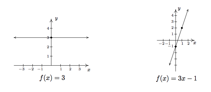
- \(f(x) = 3\)
- \(f(x) = 3x - 1\)
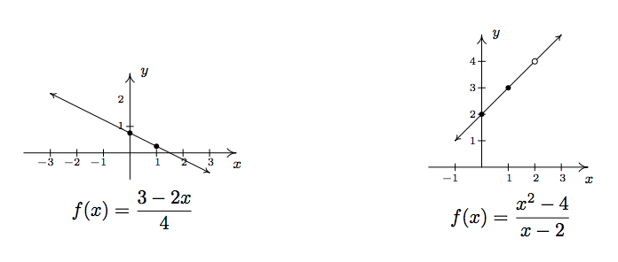
- \(f(x) = \dfrac{3 - 2x}{4}\)
- \(f(x) = \dfrac{x^2 - 4}{x-2}\)
Solution
1. To graph \(f(x) = 3\), we graph \(y=3\). This is a horizontal line \(m=0\) through \((0,3)\).
2. The graph of \(f(x) = 3x-1\) is the graph of the line \(y = 3x-1\). Comparison of this equation with Equation 2.3 yields \(m=3\) and \(b = -1\). Hence, our slope is \(3\) and our \(y\)-intercept is \((0,-1)\). To get another point on the line, we can plot \((1,f(1)) = (1,2)\).
3. At first glance, the function \(f(x) = \frac{3 - 2x}{4}\) does not fit the form in Definition 2.1 but after some rearranging we get \(f(x) = \frac{3 - 2x}{4} = \frac{3}{4} - \frac{2x}{4} = -\frac{1}{2} x + \frac{3}{4}\). We identify \(m = -\frac{1}{2}\) and \(b = \frac{3}{4}\). Hence, our graph is a line with a slope of \(-\frac{1}{2}\) and a \(y\)-intercept of \(\left(0, \frac{3}{4}\right)\). Plotting an additional point, we can choose \((1,f(1))\) to get \(\left(1, \frac{1}{4}\right)\).
4. If we simplify the expression for \(f\), we get
\[ f(x) = \dfrac{x^2-4}{x-2} = \dfrac{\cancel{(x-2)}(x+2)}{\cancel{(x-2)}} = x+2.\]
If we were to state \(f(x) = x+2\), we would be committing a sin of omission. Remember, to find the domain of a function, we do so \(\textbf{before}\) we simplify! In this case, \(f\) has big problems when \(x=2\), and as such, the domain of \(f\) is \((-\infty, 2) \cup (2,\infty)\). To indicate this, we write \(f(x) = x+2,\) \(x \neq 2\). So, except at \(x=2\), we graph the line \(y = x+2\). The slope \(m =1\) and the \(y\)-intercept is \((0,2)\). A second point on the graph is \((1,f(1)) = (1,3)\). Since our function \(f\) is not defined at \(x=2\), we put an open circle at the point that would be on the line \(y=x+2\) when \(x=2\), namely \((2,4)\).
The last two functions in the previous example showcase some of the difficulty in defining a linear function using the phrase 'of the form' as in Definition 2.1, since some algebraic manipulations may be needed to rewrite a given function to match 'the form'. Keep in mind that the domains of linear and constant functions are all real numbers \((-\infty, \infty)\), so while \(f(x) = \frac{x^2-4}{x-2}\) simplified to a formula \(f(x) = x+2\), \(f\) is not considered a linear function since its domain excludes \(x=2\). However, we would consider
\[f(x) = \dfrac{2x^2 + 2}{x^2+1}\]
to be a constant function since its domain is all real numbers (Can you tell us why?) and
\[ f(x) = \dfrac{2x^2 + 2}{x^2+1} = \dfrac{2\cancel{\left(x^2+1\right)}}{\cancel{\left(x^2+1\right)}} = 2\]
The following example uses linear functions to model some basic economic relationships.
Example \(\PageIndex{5}\):
The cost \(C\), in dollars, to produce \(x\) PortaBoy game systems for a local retailer is given by \(C(x) = 80x + 150\) for \(x \geq 0\).
- Find and interpret \(C(10)\).
- How many PortaBoys can be produced for \(\$15,\! 000\)?
- Explain the significance of the restriction on the domain, \(x \geq 0\).
- Find and interpret \(C(0)\).
- Find and interpret the slope of the graph of \(y = C(x)\).
Solution
- To find \(C(10)\), we replace every occurrence of \(x\) with \(10\) in the formula for \(C(x)\) to get \(C(10) = 80(10)+150 = 950\). Since \(x\) represents the number of PortaBoys produced, and \(C(x)\) represents the cost, in dollars, \(C(10) = 950\) means it costs \(\$950\) to produce \(10\) PortaBoys for the local retailer.
- To find how many PortaBoys can be produced for \(\$15, \! 000\), we solve \(C(x) = 15000\), or \(80x+150 = 15000\). Solving, we get \(x = \frac{14850}{80} = 185.625\). Since we can only produce a whole number amount of PortaBoys, we can produce \(185\) PortaBoys for \(\$15, \! 000\).
- The restriction \(x \geq 0\) is the applied domain, as discussed in Section 1.4. In this context, \(x\) represents the number of PortaBoys produced. It makes no sense to produce a negative quantity of game systems.\footnote{Actually, it makes no sense to produce a fractional part of a game system, either, as we saw in the previous part of this example. This absurdity, however, seems quite forgivable in some textbooks but not to us.}
- We find \(C(0) = 80(0)+150 = 150\). This means it costs \(\$150\) to produce \(0\) PortaBoys. As mentioned in Section 1.4, this is the fixed, or start-up cost of this venture.
- If we were to graph \(y = C(x)\), we would be graphing the portion of the line \(y = 80x + 150\) for \(x \geq 0\). We recognize the slope, \(m = 80\). Like any slope, we can interpret this as a rate of change. Here, \(C(x)\) is the cost in dollars, while \(x\) measures the number of PortaBoys so
\[ m = \dfrac{\Delta y}{\Delta x} = \dfrac{\Delta C}{\Delta x} = 80 = \dfrac{80}{1} = \dfrac{\\) 80}{1 \, \mbox{PortaBoy}}.\]
In other words, the cost is increasing at a rate of \(\$80\) per PortaBoy produced. This is often called the variable cost for this venture.
The next example asks us to find a linear function to model a related economic problem.
Example \(\PageIndex{6}\)
The local retailer in Example 2.1.4 has determined that the number \(x\) of PortaBoy game systems sold in a week is related to the price \(p\) in dollars of each system. When the price was \(\$220\), \(20\) game systems were sold in a week. When the systems went on sale the following week, \(40\) systems were sold at \(\$190\) a piece.
- Find a linear function which fits this data. Use the weekly sales \(x\) as the independent variable and the price \(p\) as the dependent variable.
- Find a suitable applied domain.
- Interpret the slope.
- If the retailer wants to sell \(150\) PortaBoys next week, what should the price be?
- What would the weekly sales be if the price were set at \(\$150\) per system?
Solution
- We recall from Section 1.4 the meaning of 'independent' and 'dependent' variable. Since \(x\) is to be the independent variable, and \(p\) the dependent variable, we treat \(x\) as the input variable and \(p\) as the output variable. Hence, we are looking for a function of the form \(p(x) = mx + b\). To determine \(m\) and \(b\), we use the fact that \(20\) PortaBoys were sold during the week when the price was \(220\) dollars and \(40\) units were sold when the price was \(190\) dollars. Using function notation, these two facts can be translated as \(p(20)=220\) and \(p(40)=190\). Since \(m\) represents the rate of change of \(p\) with respect to \(x\), we have \[ m = \dfrac{\Delta p}{\Delta x} = \dfrac{190-220}{40-20} = \dfrac{-30}{20} = -1.5.\] We now have determined \(p(x) = -1.5 x + b\). To determine \(b\), we can use our given data again. Using \(p(20) = 220\), we substitute \(x=20\) into \(p(x) = 1.5x + b\) and set the result equal to \(220\): \(-1.5(20)+b = 220\). Solving, we get \(b = 250\). Hence, we get \(p(x) = -1.5x + 250\). We can check our formula by computing \(p(20)\) and \(p(40)\) to see if we get \(220\) and \(190\), respectively. You may recall from Section 1.5 that the function \(p(x)\) is called the price-demand (or simply demand) function for this venture.
- To determine the applied domain, we look at the physical constraints of the problem. Certainly, we can't sell a negative number of PortaBoys, so \(x \geq 0\). However, we also note that the slope of this linear function is negative, and as such, the price is decreasing as more units are sold. Thus another constraint on the price is \(p(x)\geq 0\). Solving \(-1.5 x + 250 \geq 0\) results in \(-1.5 x \geq -250\) or \(x \leq \dfrac{500}{3} = 166.\overline{6}\). Since \(x\) represents the number of PortaBoys sold in a week, we round down to \(166\). As a result, a reasonable applied domain for \(p\) is \([0,166]\).
- The slope \(m = -1.5\), once again, represents the rate of change of the price of a system with respect to weekly sales of PortaBoys. Since the slope is negative, we have that the price is decreasing at a rate of \(\$1.50\) per PortaBoy sold. (Said differently, you can sell one more PortaBoy for every \(\$1.50\) drop in price.)
- To determine the price which will move \(150\) PortaBoys, we find \(p(150) = -1.5(150) + 250 = 25\). That is, the price would have to be \(\$25\).
- If the price of a PortaBoy were set at \(\$150\), we have \(p(x) = 150\), or, \(-1.5x + 250 = 150\). Solving, we get \(-1.5x = -100\) or \(x = 66.\overline{6}\). This means you would be able to sell \(66\) PortaBoys a week if the price were \(\$150\) per system.
Not all real-world phenomena can be modeled using linear functions. Nevertheless, it is possible to use the concept of slope to help analyze non-linear functions using the following.
Definition 2.3: Average Rate of Change
Let \(f\) be a function defined on the interval \([a,b]\). The average rate of change of \(f\) over \([a,b]\) is defined as: \[ \dfrac{\Delta f}{\Delta x} = \dfrac{f(b) - f(a)}{b-a} \]
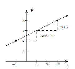
Geometrically, if we have the graph of \(y=f(x)\), the average rate of change over \([a,b]\) is the slope of the line which connects \((a,f(a))\) and \((b,f(b))\). This is called the secant line through these points. For that reason, some textbooks use the notation \(m_{\sec}\) for the average rate of change of a function. Note that for a linear function \(m = m_{\sec}\), or in other words, its rate of change over an interval is the same as its average rate of change.
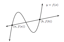
The graph of \(y=f(x)\) and its secant line through \((a,f(a))\) and \((b,f(b))\)
The interested reader may question the adjective 'average' in the phrase 'average rate of change'. In the figure above, we can see that the function changes wildly on \([a,b]\), yet the slope of the secant line only captures a snapshot of the action at \(a\) and \(b\). This situation is entirely analogous to the average speed on a trip. Suppose it takes you \(2\) hours to travel \(100\) miles. Your average speed is \(\frac{100 \, \mbox{ miles}}{2 \, \mbox{ hours}} = 50 \, \mbox{miles per hour}\). However, it is entirely possible that at the start of your journey, you traveled \(25\) miles per hour, then sped up to \(65\) miles per hour, and so forth. The average rate of change is akin to your average speed on the trip. Your speedometer measures your speed at any one instant along the trip, your instantaneous rate of change, and this is one of the central themes of Calculus.
When interpreting rates of change, we interpret them the same way we did slopes. In the context of functions, it may be helpful to think of the average rate of change as:
\[ \dfrac{\mbox{change in outputs}}{\mbox{change in inputs}}\]
Example \(\PageIndex{7}\):
Recall from Section 1.5, the revenue from selling \(x\) units at a price \(p\) per unit is given by the formula \(R=xp\). Suppose we are in the scenario of Examples 2.1.5 and 2.1.6.
- Find and simplify an expression for the weekly revenue \(R(x)\) as a function of weekly sales \(x\).
- Find and interpret the average rate of change of \(R(x)\) over the interval \([0,50]\).
- Find and interpret the average rate of change of \(R(x)\) as \(x\) changes from \(50\) to \(100\) and compare that to your result in part 2.
- Find and interpret the average rate of change of weekly revenue as weekly sales increase from \(100\) PortaBoys to \(150\) PortaBoys.
Solution
- Since \(R = xp\), we substitute \(p(x) = -1.5x + 250\) from Example 2.1.6 to get \(R(x) = x (-1.5x + 250) = -1.5x^2+250x\). Since we determined the price-demand function \(p(x)\) is restricted to \(0 \leq x \leq 166\), \(R(x)\) is restricted to these values of \(x\) as well.
- Using Definition 2.3, we get that the average rate of change is \[ \dfrac{\Delta R}{\Delta x} = \dfrac{R(50) - R(0)}{50 - 0} = \dfrac{8750 - 0}{50 - 0} = 175.\]
- Interpreting this slope as we have in similar situations, we conclude that for every additional PortaBoy sold during a given week, the weekly revenue increases \(\$ 175\).
- The wording of this part is slightly different than that in Definition 2.3, but its meaning is to find the average rate of change of \(R\) over the interval \([50,100]\). To find this rate of change, we compute \[ \dfrac{\Delta R}{\Delta x} = \dfrac{R(100) - R(50)}{100-50} = \dfrac{10000 - 8750}{50} = 25.\] In other words, for each additional PortaBoy sold, the revenue increases by \(\$25\). Note that while the revenue is still increasing by selling more game systems, we aren't getting as much of an increase as we did in part 2 of this example. (Can you think of why this would happen?)
- Translating the English to the mathematics, we are being asked to find the average rate of change of \(R\) over the interval \([100,150]\). We find \[ \dfrac{\Delta R}{\Delta x} = \dfrac{R(150) - R(100)}{150-100} = \dfrac{3750 - 10000}{50} = -125.\] This means that we are losing \(\$125\) dollars of weekly revenue for each additional PortaBoy sold. (Can you think why this is possible?)
We close this section with a new look at difference quotients which were first introduced in Section 1.4. If we wish to compute the average rate of change of a function \(f\) over the interval \([x, x+h]\), then we would have
\[ \dfrac{\Delta f}{\Delta x} = \dfrac{f(x+h) - f(x)}{(x+h) - x} = \dfrac{f(x+h) - f(x)}{h}\]
As we have indicated, the rate of change of a function (average or otherwise) is of great importance in Calculus.\footnote{So we are not torturing you with these for nothing.} Also, we have the geometric interpretation of difference quotients which was promised to you back in Section 1.5 -- a difference quotient yields the slope of a secant line.