3.5: Real Zeros of Polynomials

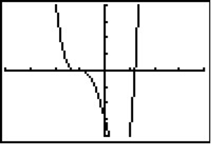
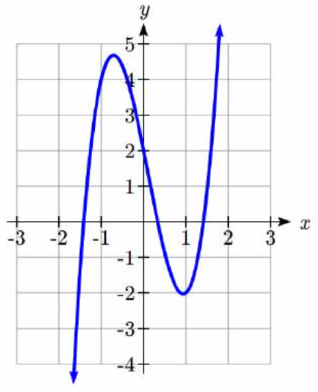
In the last section, we saw how to determine if a real number was a zero of a polynomial. In this section, we will learn how to find good candidates to test using synthetic division. In the days before graphing technology was commonplace, mathematicians discovered a lot of clever tricks for determining the likely locations of zeros. Technology has provided a much simpler approach to narrow down potential candidates, but it is not always sufficient by itself. For example, the function shown to the right does not have any clear intercepts.

There are two results that can help us identify where the zeros of a polynomial are. The first gives us an interval on which all the real zeros of a polynomial can be found.

Definition: Cauchy’s Bound

Given a polynomial

\[(f(x)=a_{n} x^{n} +a_{n-1} x^{n-1} +\cdots +a_{1} x+a_{0},\]

let \(M\) be the largest of the coefficients in absolute value. Then all the real zeros of \(f(x)\) lie in the interval

\[\left[-\dfrac{M}{\left|a_{n} \right|} -1,\quad \dfrac{M}{\left|a_{n} \right|} +1\right] \label{Cauchy}\]

Example 1

Let \(f(x)=2x^{4} +4x^{3} -x^{2} -6x-3\). Determine an interval which contains all the real zeros of f.

Solution

To find the \(M\) from Cauchy’s Bound, we take the absolute value of the coefficients and pick the largest, in this case \(\left|-6\right|=6\). Divide this by the absolute value of the leading coefficient, 2, to get 3. All the real zeros of f lie in the interval

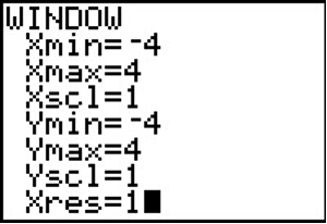
\[\left[-\dfrac{6}{\left|2\right|} -1,\quad \dfrac{6}{\left|2\right|} +1\right]=\left[-3-1,\quad 3+1\right]=[-4,\; 4]. \nonumber\]

Knowing this bound can be very helpful when using a graphing calculator, since we can use it to set the display bounds. This helps avoid missing a zero because it is graphed outside of the viewing window.

Exercise \(\PageIndex{1}\)

Determine an interval which contains all the real zeros of \(f(x)=3x^{3} -12x^{2} +6x-8\).

Answer

The maximum coefficient in absolute value is 12. Cauchy’s Bound for all real zeros is

\[\left[-\dfrac{12}{\left|3\right|} -1,\quad \dfrac{12}{\left|3\right|} +1\right]=[-5,5]\nonumber \]

Now that we know where we can find the real zeros, we still need a list of possible real zeros. The Rational Roots Theorem provides us a list of potential integer and rational zeros.

rational roots theorem

Given a polynomial

\[f(x)=a_{n} x^{n} +a_{n-1} x^{n-1} +\cdots +a_{1} x+a_{0}\]

with integer coefficients, if \(r\) is a rational zero of \(f\), then \(r\) is of the form \(r=\pm \dfrac{p}{q}\), where \(p\) is a factor of the constant term \(a_{0}\), and \(q\) is a factor of the leading coefficient, \(a_{n}\).

This gives us a list of numbers to try in our synthetic division, which is a nicer place to start than simply guessing. If none of the numbers in the list are zeros, then either the polynomial has no real zeros at all, or all the real zeros are irrational numbers.

Example \(\PageIndex{2}\)

Let \(f(x)=2x^{4} +4x^{3} -x^{2} -6x-3\). Use the Rational Roots Theorem to list all the possible rational zeros of \(f(x)\).

Solution

To generate a complete list of rational zeros, we need to take each of the factors of the

constant term, \(a_{0} =-3\), and divide them by each of the factors of the leading coefficient \(a_{4} =2\). The factors of -3 are \(\pm 1\) and \(\pm 3\). Since the Rational Roots Theorem tacks on a \(\pm\) anyway, for the moment, we consider only the positive factors 1 and 3. The factors of 2 are 1 and 2, so the Rational Roots Theorem gives the list

\[\left\{\pm \dfrac{1}{1} ,\pm \dfrac{1}{2} ,\pm \dfrac{3}{1} ,\pm \dfrac{3}{2} \right\}\text{ ,or }\left\{\pm 1,\pm \dfrac{1}{2} ,\pm 3,\pm \dfrac{3}{2} \right\}\nonumber \]

Now we can use synthetic division to test these possible zeros. To narrow the list first, we could use graphing technology to help us identify some good possibilities.

Example \(\PageIndex{3}\)

Find the horizontal intercepts of \(f(x)=2x^{4} +4x^{3} -x^{2} -6x-3\).

Solution

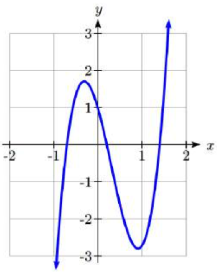
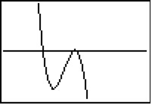
From Example 1, we know that the real zeros lie in the interval [-4, 4]. Using a graphing calculator, we could set the window accordingly and get the graph below.

                

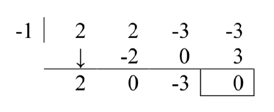
In Example 2, we learned that any rational zero must be on the list \(\left\{\pm 1,\pm \dfrac{1}{2} ,\pm 3,\pm \dfrac{3}{2} \right\}\). From the graph, it looks like -1 is a good possibility, so we try that using synthetic division.

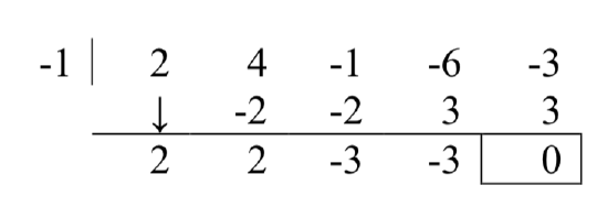
Success! Remembering that \(f\) was a fourth degree polynomial, we know that our quotient is a third degree polynomial. If we can do one more successful division, we will have knocked the quotient down to a quadratic, and, if all else fails, we can use the quadratic formula to find the last two zeros. Since there seems to be no other rational zeros to try, we continue with -1. Also, the shape of the crossing at \(x = -1\) leads us to wonder if the zero \(x = -1\) has multiplicity 3.

Success again! Our quotient polynomial is now \(2x^{2} -3\). Setting this to zero gives \(2x^{2} -3=0\), giving \(x=\pm \sqrt{\dfrac{3}{2} } =\pm \dfrac{\sqrt{6} }{2}\). Since a fourth degree polynomial can have at most four zeros, including multiplicities, then the intercept x = -1 must only have multiplicity 2, which we had found through division, and not 3 as we had guessed.

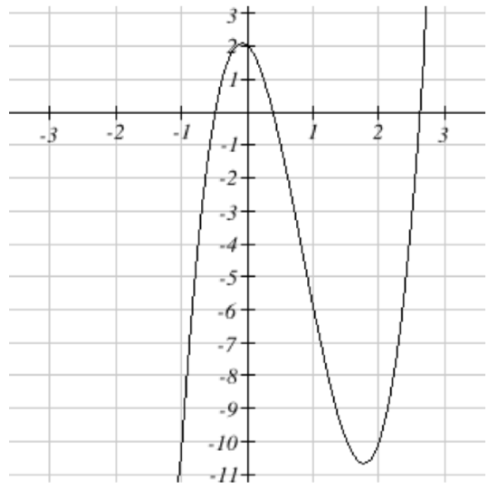
It is interesting to note that we could greatly improve on the graph of \(y=f(x)\)in the previous example given to us by the calculator. For instance, from our determination of the zeros of \(f\) and their multiplicities, we know the graph crosses at \(x=-\dfrac{\sqrt{6} }{2} \approx -1.22\) then turns back upwards to touch the \(x\)-axis at \(x = -1\). This tells us that, despite what the calculator showed us the first time, there is a relative maximum occurring at \(x = -1\) and not a "flattened crossing" as we originally believed.

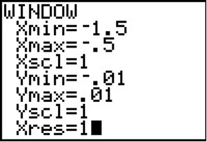
After resizing the window, we see not only the relative maximum but also a relative minimum just to the left of \(x = -1\)

                        

In this case, mathematics helped reveal something that was hidden in the initial graph.

Example 4

Find the real zeros of \(f(x)=4x^{3} -10x^{2} -2x+2\).

Solution

Cauchy’s Bound tells us that the real zeros lie in the interval \(\left[-\dfrac{10}{\left|4\right|} -1,\quad \dfrac{10}{\left|4\right|} +1\right]=[-3.5,\; 3.5]\).

Graphing on this interval reveals no clear integer zeros. Turning to the rational roots theorem, we need to take each of the factors of the constant term, \(a_{0} =2\), and divide them by each of the factors of the leading coefficient \(a_{3} =4\). The factors of 2 are 1 and 2. The factors of 4 are 1, 2, and 4, so the Rational Roots Theorem gives the list

\[\left\{\pm \dfrac{1}{1} ,\pm \dfrac{1}{2} ,\pm \dfrac{1}{4} ,\pm \dfrac{2}{1} ,\pm \dfrac{2}{2} ,\pm \dfrac{2}{4} \right\}\text{ ,or }\left\{\pm 1,\pm \dfrac{1}{2} ,\pm \dfrac{1}{4} ,\pm 2\right\}\nonumber \]

The two most likely candidates are \(\pm \dfrac{1}{2}\).

Trying \(\dfrac{1}{2}\),

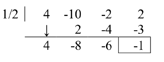
The remainder is not zero, so this is not a zero. Trying \(-\dfrac{1}{2}\),

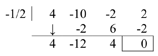
Success! This tells us \(4x^{3} -10x^{2} -2x+2=\left(x+\dfrac{1}{2} \right)\left(4x^{2} -12x+4\right)\), and that the graph has a horizontal intercept at \(x=-\dfrac{1}{2}\).

To find the remaining two intercepts, we can use the quadratic equation, setting \(4x^{2} -12x+4=0\). First, we might pull out the common factor, \(4\left(x^{2} -3x+1\right)=0\).

\[x=\dfrac{3\pm \sqrt{(-3)^{2} -4(1)(1)} }{2(1)} =\dfrac{3\pm \sqrt{5} }{2} \approx 2.618,\; \; 0.382\nonumber \]

Exercise \(\PageIndex{2}\)

Find the real zeros of \(f(x)=3x^{3} -x^{2} -6x+2\)

Answer

Cauchy’s Bound tells us the zeros lie in the interval \(\left[-\dfrac{6}{\left|3\right|} -1,\quad \dfrac{6}{\left|3\right|} +1\right]=[-3,3]\). The rational roots theorem tells us the possible rational zeros of the polynomial are on the list

\[\left\{\pm \dfrac{1}{1} ,\pm \dfrac{1}{3} ,\pm \dfrac{2}{1} ,\pm \dfrac{2}{3} \right\}=\left\{\pm 1,\pm \dfrac{1}{3} ,\pm 2,\pm \dfrac{2}{3} \right\}\nonumber \]

Looking at a graph, the only likely candidate is \(\dfrac{1}{3}\)

Using synthetic division,

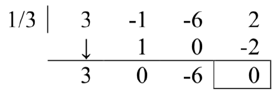
\[3x^{3} -x^{2} -6x+2=\left(x-\dfrac{1}{3} \right)\left(3x^{2} -6\right)=3\left(x-\dfrac{1}{3} \right)\left(x^{2} -2\right)\nonumber \]

Solving \(x^{2} -2=0\) gives zeros \(x=\pm \sqrt{2}\).

The real zeros of the polynomial are \(x=\sqrt{2} ,\; -\sqrt{2} ,\; \dfrac{1}{3}\).

Important Topics of this Section

• Cauchy’s Bound for all real zeros of a polynomial
• Rational Roots Theorem
• Finding real zeros of a polynomial