
4.1: Number Line Graphs
- Page ID
- 83126

\( \newcommand{\vecs}[1]{\overset { \scriptstyle \rightharpoonup} {\mathbf{#1}} } \)
\( \newcommand{\vecd}[1]{\overset{-\!-\!\rightharpoonup}{\vphantom{a}\smash {#1}}} \)
\( \newcommand{\id}{\mathrm{id}}\) \( \newcommand{\Span}{\mathrm{span}}\)
( \newcommand{\kernel}{\mathrm{null}\,}\) \( \newcommand{\range}{\mathrm{range}\,}\)
\( \newcommand{\RealPart}{\mathrm{Re}}\) \( \newcommand{\ImaginaryPart}{\mathrm{Im}}\)
\( \newcommand{\Argument}{\mathrm{Arg}}\) \( \newcommand{\norm}[1]{\| #1 \|}\)
\( \newcommand{\inner}[2]{\langle #1, #2 \rangle}\)
\( \newcommand{\Span}{\mathrm{span}}\)
\( \newcommand{\id}{\mathrm{id}}\)
\( \newcommand{\Span}{\mathrm{span}}\)
\( \newcommand{\kernel}{\mathrm{null}\,}\)
\( \newcommand{\range}{\mathrm{range}\,}\)
\( \newcommand{\RealPart}{\mathrm{Re}}\)
\( \newcommand{\ImaginaryPart}{\mathrm{Im}}\)
\( \newcommand{\Argument}{\mathrm{Arg}}\)
\( \newcommand{\norm}[1]{\| #1 \|}\)
\( \newcommand{\inner}[2]{\langle #1, #2 \rangle}\)
\( \newcommand{\Span}{\mathrm{span}}\) \( \newcommand{\AA}{\unicode[.8,0]{x212B}}\)
\( \newcommand{\vectorA}[1]{\vec{#1}} % arrow\)
\( \newcommand{\vectorAt}[1]{\vec{\text{#1}}} % arrow\)
\( \newcommand{\vectorB}[1]{\overset { \scriptstyle \rightharpoonup} {\mathbf{#1}} } \)
\( \newcommand{\vectorC}[1]{\textbf{#1}} \)
\( \newcommand{\vectorD}[1]{\overrightarrow{#1}} \)
\( \newcommand{\vectorDt}[1]{\overrightarrow{\text{#1}}} \)
\( \newcommand{\vectE}[1]{\overset{-\!-\!\rightharpoonup}{\vphantom{a}\smash{\mathbf {#1}}}} \)
\( \newcommand{\vecs}[1]{\overset { \scriptstyle \rightharpoonup} {\mathbf{#1}} } \)
\( \newcommand{\vecd}[1]{\overset{-\!-\!\rightharpoonup}{\vphantom{a}\smash {#1}}} \)
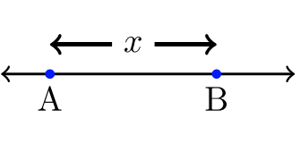
\(\newcommand{\avec}{\mathbf a}\) \(\newcommand{\bvec}{\mathbf b}\) \(\newcommand{\cvec}{\mathbf c}\) \(\newcommand{\dvec}{\mathbf d}\) \(\newcommand{\dtil}{\widetilde{\mathbf d}}\) \(\newcommand{\evec}{\mathbf e}\) \(\newcommand{\fvec}{\mathbf f}\) \(\newcommand{\nvec}{\mathbf n}\) \(\newcommand{\pvec}{\mathbf p}\) \(\newcommand{\qvec}{\mathbf q}\) \(\newcommand{\svec}{\mathbf s}\) \(\newcommand{\tvec}{\mathbf t}\) \(\newcommand{\uvec}{\mathbf u}\) \(\newcommand{\vvec}{\mathbf v}\) \(\newcommand{\wvec}{\mathbf w}\) \(\newcommand{\xvec}{\mathbf x}\) \(\newcommand{\yvec}{\mathbf y}\) \(\newcommand{\zvec}{\mathbf z}\) \(\newcommand{\rvec}{\mathbf r}\) \(\newcommand{\mvec}{\mathbf m}\) \(\newcommand{\zerovec}{\mathbf 0}\) \(\newcommand{\onevec}{\mathbf 1}\) \(\newcommand{\real}{\mathbb R}\) \(\newcommand{\twovec}[2]{\left[\begin{array}{r}#1 \\ #2 \end{array}\right]}\) \(\newcommand{\ctwovec}[2]{\left[\begin{array}{c}#1 \\ #2 \end{array}\right]}\) \(\newcommand{\threevec}[3]{\left[\begin{array}{r}#1 \\ #2 \\ #3 \end{array}\right]}\) \(\newcommand{\cthreevec}[3]{\left[\begin{array}{c}#1 \\ #2 \\ #3 \end{array}\right]}\) \(\newcommand{\fourvec}[4]{\left[\begin{array}{r}#1 \\ #2 \\ #3 \\ #4 \end{array}\right]}\) \(\newcommand{\cfourvec}[4]{\left[\begin{array}{c}#1 \\ #2 \\ #3 \\ #4 \end{array}\right]}\) \(\newcommand{\fivevec}[5]{\left[\begin{array}{r}#1 \\ #2 \\ #3 \\ #4 \\ #5 \\ \end{array}\right]}\) \(\newcommand{\cfivevec}[5]{\left[\begin{array}{c}#1 \\ #2 \\ #3 \\ #4 \\ #5 \\ \end{array}\right]}\) \(\newcommand{\mattwo}[4]{\left[\begin{array}{rr}#1 \amp #2 \\ #3 \amp #4 \\ \end{array}\right]}\) \(\newcommand{\laspan}[1]{\text{Span}\{#1\}}\) \(\newcommand{\bcal}{\cal B}\) \(\newcommand{\ccal}{\cal C}\) \(\newcommand{\scal}{\cal S}\) \(\newcommand{\wcal}{\cal W}\) \(\newcommand{\ecal}{\cal E}\) \(\newcommand{\coords}[2]{\left\{#1\right\}_{#2}}\) \(\newcommand{\gray}[1]{\color{gray}{#1}}\) \(\newcommand{\lgray}[1]{\color{lightgray}{#1}}\) \(\newcommand{\rank}{\operatorname{rank}}\) \(\newcommand{\row}{\text{Row}}\) \(\newcommand{\col}{\text{Col}}\) \(\renewcommand{\row}{\text{Row}}\) \(\newcommand{\nul}{\text{Nul}}\) \(\newcommand{\var}{\text{Var}}\) \(\newcommand{\corr}{\text{corr}}\) \(\newcommand{\len}[1]{\left|#1\right|}\) \(\newcommand{\bbar}{\overline{\bvec}}\) \(\newcommand{\bhat}{\widehat{\bvec}}\) \(\newcommand{\bperp}{\bvec^\perp}\) \(\newcommand{\xhat}{\widehat{\xvec}}\) \(\newcommand{\vhat}{\widehat{\vvec}}\) \(\newcommand{\uhat}{\widehat{\uvec}}\) \(\newcommand{\what}{\widehat{\wvec}}\) \(\newcommand{\Sighat}{\widehat{\Sigma}}\) \(\newcommand{\lt}{<}\) \(\newcommand{\gt}{>}\) \(\newcommand{\amp}{&}\) \(\definecolor{fillinmathshade}{gray}{0.9}\)A real number line is a visual approach to ordering all real numbers:
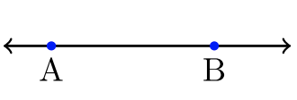
Any real number \(A\) plotted left of another real number \(B\) has the relation: \(A < B\), or equivalently, \(B > A\). We read aloud, “\(A\) is less than \(B\)” or equivalently, “\(B\) is greater than \(A\).”
Graphing Inequalities
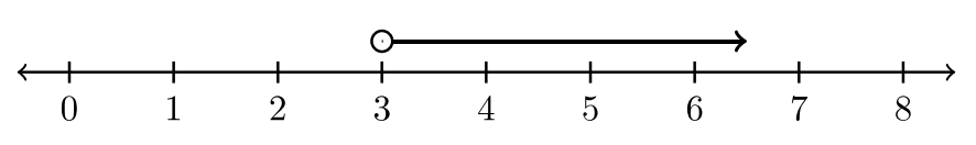
“Graph the solution set, \(x > 3\).”
The solution set to an inequality is the set of real numbers that make the inequality a true statement. All values that lie to the right of \(3\) on the number line are greater than \(3\). The number \(3\) itself is not greater than \(3\). A graph quickly conveys the solution set. To visually denote that \(3\) is not greater than \(3\), we will use an open circled; a circle that is not filled. The blue portion of this number line indicates values greater than \(3\).
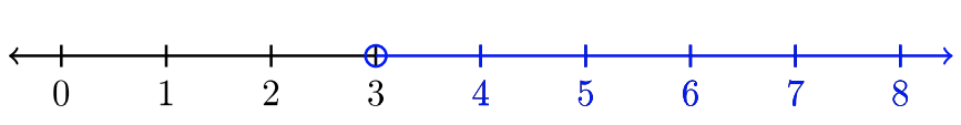
Finally, we shift the entire blue line above the number line. Now we don’t need colors:
All values \(x > 3\) are graphed below:
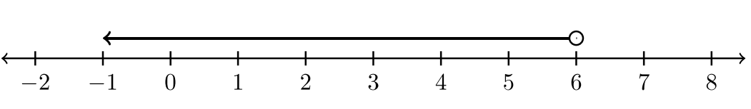
Graph the solution set \(y < 6\).
Solution
The solution set is the set of all real numbers strictly less than \(6\). The number line graph conveys the solution:
How to Decide: Closed or Open Circle?
| Inequality | Associated Circle | Example Graphs |
|---|---|---|
|
Either \(<\) or \(>\) |
 |
\(x < 1\)
|
|
Either \(≤\) or \(≥\) |
 |
\(x ≤ 1\)
|
Graph the solution set of \(−4 ≤ t\).
Solution
The given inequality is equivalent to \(t ≥ −4\). The graph will express all values greater than or equal to \(−4\). In this case, \(−4\) is included as a solution. Use a filled circle to denote its inclusion in the solution set.
All Values Between A and B: Compound Inequalities
If we want to describe all numbers between \(A\) and \(B\), there is an elegant way to do this. Let \(x =\) all real numbers between \(A\) and \(B\). The examples below use \(A = –2\) and \(B = 3\). The open and closed circles correspond with the appropriate inequality.
| Inequality | Graph | ||
|---|---|---|---|
| \(– 2 < x < 3\) | 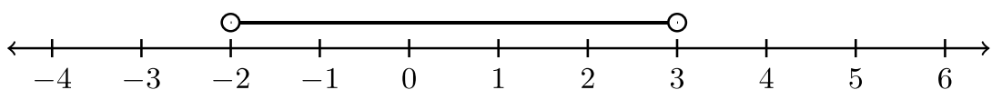 |
||
| \(– 2 < x ≤ 3\) | 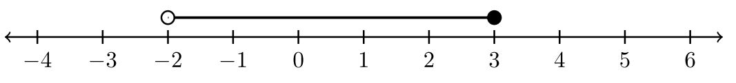 |
||
| \(– 2 ≤ x < 3\) | 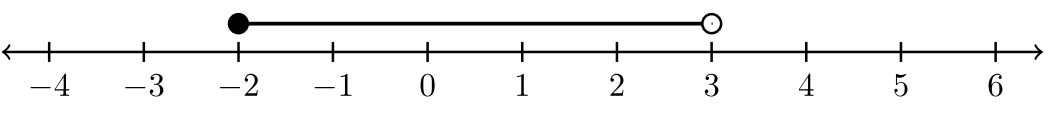 |
||
| \(−2 ≤ x ≤ 3\) | 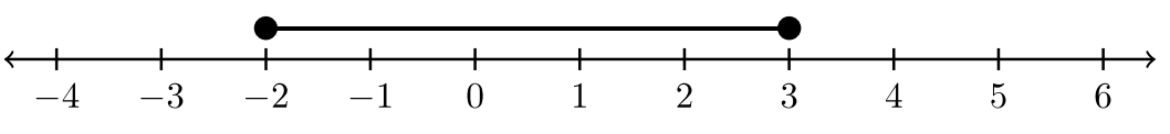 |
||
These inequalities are handled no differently, yet the unit is \(π\):
| Inequality | Graph | ||
|---|---|---|---|
| \(– 2 \pi ≤ x ≤ 2 \pi\) | 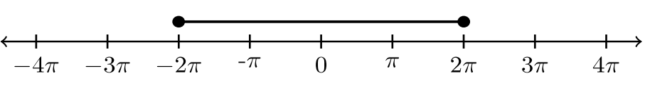 |
||
| \(−4 \pi ≤ x < 0\) | 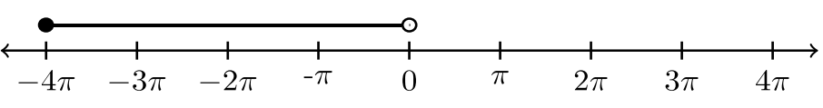 |
||
| \(0 < x ≤ 3 \pi\) | 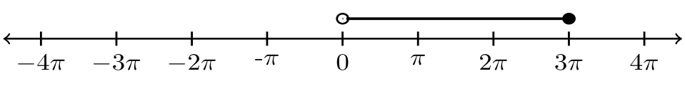 |
||
| \(−\pi < x < \pi\) | 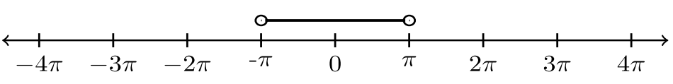 |
||
Compound Inequalities
The above inequalities are examples of compound inequalities: inequalities that express two or more inequalities at once. We can split each inequality above into two inequalities, using an “and” statement between each inequality:
\(A < x < B\) is equivalent to \(A < x\) and \(x < B\)
Notice \(A < B\). When the inequalities are uncoupled, the middle variable is expressed in both inequalities, and the inequality symbol is maintained.
We’ll revisit compound inequalities in the context of absolute value inequalities in Section 4.4.
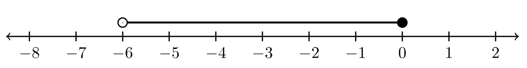
Graph the solution set of the compound inequality: \(x > −6\) and \(x ≤ 0\).
Solution
The two inequalities have an “and” statement between them. The first inequality \(x > −6\) can be restated in its equivalent form: \(−6 < x\). The real value \(A = −6\) is the left endpoint, whereas \(B = 0\) is the right endpoint. The graph is shown below for \(−6 < x ≤ 0\).
Try It! (Exercises)
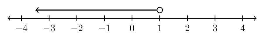
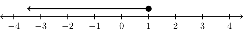
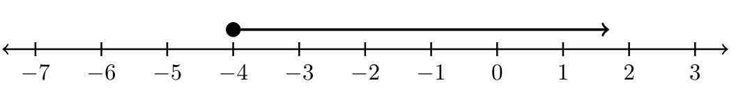
For exercises #1-10, state the inequality that is represented by the graph.
| Inequality | Graph | ||
|---|---|---|---|
| 1. |  |
||
| 2. |  |
||
| 3. |  |
||
| 4. | 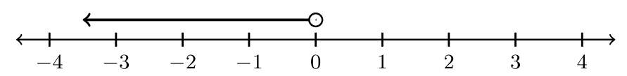 |
||
| 5. | 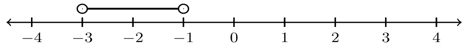 |
||
| 6. | 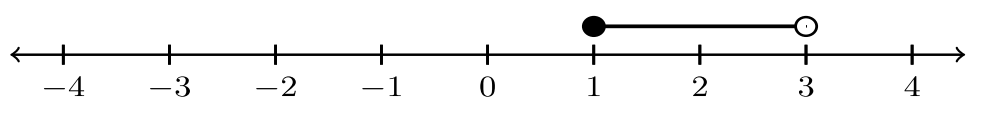 |
||
| 7. | 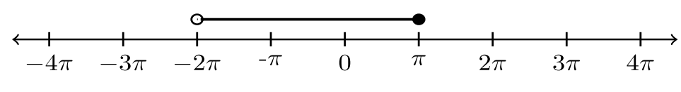 |
||
| 8. | 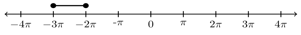 |
||
| 9. | 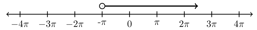 |
||
| 10. | 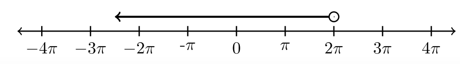 |
||
For exercises #11-15, the number line is equally divided. Label the tick marks. Use fractions. Then sketch the number line graph that represents each inequality.
| Inequality | Graph | ||
|---|---|---|---|
| 11. \(-\dfrac{1}{2} < x ≤ \dfrac{3}{2}\) | 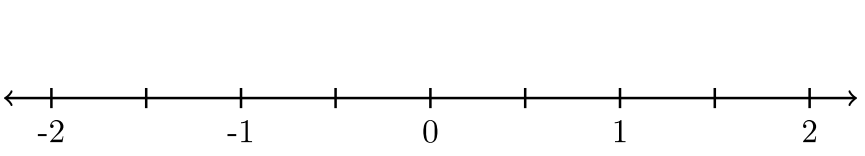 |
||
| 12. \(x ≥ \dfrac{1}{2}\) | 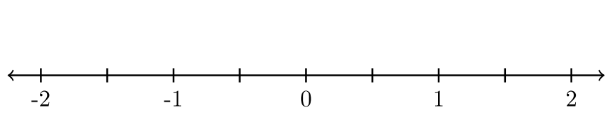 |
||
| 13. \(x < −\dfrac{3}{2}\) | 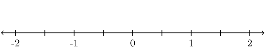 |
||
| 14. \(−\dfrac{3 \pi}{2} ≤ x < \dfrac{3 \pi}{2}\) | 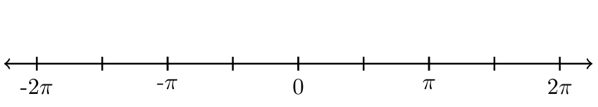 |
||
| 15. \(−\dfrac{\pi}{4} < x < \dfrac{3 \pi}{4}\) | 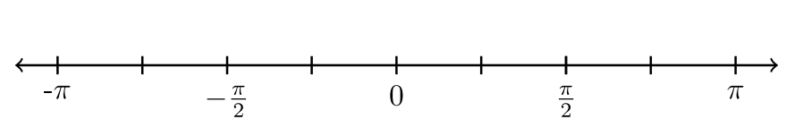 |
||
For exercises #16-22, Sketch a number line graph that corresponds with the given compound inequality.
- \(x > −2\) and \(x ≤ 5\)
- \(x ≥ 1\) and \(x ≤ 10\)
- \(x ≤ −1\) and \(x > −3\)
- \(x < 8\) and \(x ≥ −8\)
- \(x > −\dfrac{3}{2}\) and \(x < \dfrac{1}{2}\)
- \(x ≥ 2 \pi\) and \(x ≤ 4 \pi\)
- \(x > −\dfrac{\pi}{2}\) and \(x < \dfrac{\pi}{2}\)