
12.1: Finding Limits - Numerical and Graphical Approaches


- Last updated
- Jan 2, 2021
- Save as PDF

( \newcommand{\kernel}{\mathrm{null}\,}\)
Intuitively, we know what a limit is. A car can go only so fast and no faster. A trash can might hold 33 gallons and no more. It is natural for measured amounts to have limits. What, for instance, is the limit to the height of a woman? The tallest woman on record was Jinlian Zeng from China, who was 8 ft 1 in.1 Is this the limit of the height to which women can grow? Perhaps not, but there is likely a limit that we might describe in inches if we were able to determine what it was.
To put it mathematically, the function whose input is a woman and whose output is a measured height in inches has a limit. In this section, we will examine numerical and graphical approaches to identifying limits.
Understanding Limit Notation
We have seen how a sequence can have a limit, a value that the sequence of terms moves toward as the nu mber of terms increases. For example, the terms of the sequence
1,12,14,18...
gets closer and closer to 0. A sequence is one type of function, but functions that are not sequences can also have limits. We can describe the behavior of the function as the input values get close to a specific value. If the limit of a function f(x)=L, then as the input x gets closer and closer to a, the output y-coordinate gets closer and closer to L. We say that the output “approaches” L.
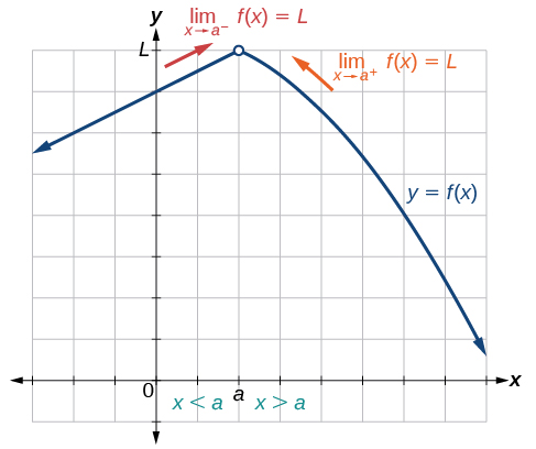
Figure 12.1.1 provides a visual representation of the mathematical concept of limit. As the input value x approaches a, the output value f(x) approaches L.
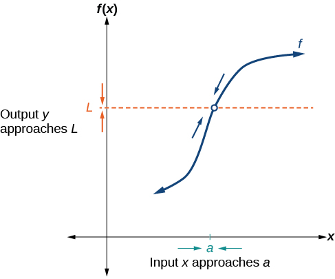
We write the equation of a limit as
limx→af(x)=L.
This notation indicates that as x approaches a both from the left of x=a and the right of x=a, the output value approaches L.
Consider the function
f(x)=x2−6x−7x−7.
We can factor the function in Equation ??? as shown.
f(x)=(x−7)(x+1)x−7Cancel like factors in numerator and denominator.f(x)=x+1,x≠7Simplify.
Notice that x cannot be 7, or we would be dividing by 0, so 7 is not in the domain of the function in Equation ???. To avoid changing the function when we simplify, we set the same condition, x≠7, for the simplified function. We can represent the function graphically as shown in Figure 12.1.2.
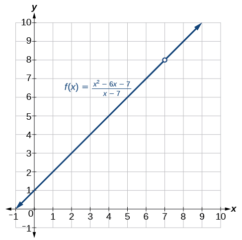
What happens at x=7 is completely different from what happens at points close to x=7 on either side. The notation
limx→7f(x)=8
indicates that as the input x approaches 7 from either the left or the right, the output approaches 8. The output can get as close to 8 as we like if the input is sufficiently near 7.
What happens at x=7? When x=7, there is no corresponding output. We write this as
f(7)does not exist.
This notation indicates that 7 is not in the domain of the function. We had already indicated this when we wrote the function as
f(x)=x+1,x≠7.
Notice that the limit of a function can exist even when f(x) is not defined at x=a. Much of our subsequent work will be determining limits of functions as x nears a, even though the output at x=a does not exist.
THE LIMIT OF A FUNCTION
A quantity L is the limit of a function f(x) as x approaches a if, as the input values of x approach a (but do not equal a),the corresponding output values of f(x) get closer to L. Note that the value of the limit is not affected by the output value of f(x) at a. Both a and L must be real numbers. We write it as
limx→af(x)=L
Example 12.1.1: Understanding the Limit of a Function
For the following limit, define a,f(x), and L.
limx→2(3x+5)=11
Solution
First, we recognize the notation of a limit. If the limit exists, as x approaches a, we write
limx→af(x)=L.
We are given
limx→2(3x+5)=11.
This means that a=2,f(x)=3x+5, and L=11.
Analysis
Recall that y=3x+5 is a line with no breaks. As the input values approach 2, the output values will get close to 11. This may be phrased with the equation limx→2(3x+5)=11, which means that as x nears 2 (but is not exactly 2), the output of the function f(x)=3x+5 gets as close as we want to 3(2)+5, or 11, which is the limit L, as we take values of x sufficiently near 2 but not at x=2.
Exercise 12.1.1
For the following limit, define a,f(x), and L.
limx→5(2x2−4)=46
Solution
a=5,f(x)=2x2−4, and L=46.
Understanding Left-Hand Limits and Right-Hand Limits
We can approach the input of a function from either side of a value—from the left or the right. Figure 12.1.3 shows the values of
f(x)=x+1,x≠7
as described earlier and depicted in Figure 12.1.3.
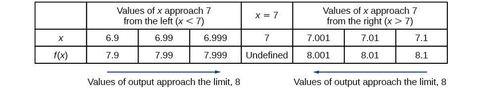
Values described as “from the right” are greater than the input value 7 and would therefore appear to the right of the value on a number line. The input values that approach 7 from the right in Figure 12.1.3 are 7.1,7.01, and 7.001. The corresponding outputs are 8.1,8.01, and 8.001. These values are getting closer to 8. The limit of values of f(x) as x approaches from the right is known as the right-hand limit. For this function, 8 is also the right-hand limit of the function f(x)=x+1,x≠7 as x approaches 7.
Figure 12.1.3 shows that we can get the output of the function within a distance of 0.1 from 8 by using an input within a distance of 0.1 from 7. In other words, we need an input x within the interval 6.9<x<7.1 to produce an output value of f(x) within the interval 7.9<f(x)<8.1.
We also see that we can get output values of f(x) successively closer to 8 by selecting input values closer to 7. In fact, we can obtain output values within any specified interval if we choose appropriate input values.
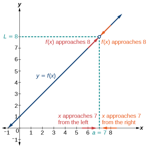
Figure 12.1.4 provides a visual representation of the left- and right-hand limits of the function. From the graph of f(x), we observe the output can get infinitesimally close to L=8 as x approaches 7 from the left and as x approaches 7 from the right.
To indicate the left-hand limit, we write
limx→7−f(x)=8.
To indicate the right-hand limit, we write
limx→7+f(x)=8.
LEFT- AND RIGHT-HAND LIMITS
The left-hand limit of a function f(x) as x approaches a from the left is equal to L, denoted by limx→a−f(x)=L.
The values of f(x) can get as close to the limit L as we like by taking values of x sufficiently close to a such that x<a and x≠a.
The right-hand limit of a function f(x), as x approaches a from the right, is equal to L, denoted by limx→a+f(x)=L.
The values of f(x) can get as close to the limit L as we like by taking values of x sufficiently close to a but greater than a. Both a and L are real numbers.
Understanding Two-Sided Limits
In the previous example, the left-hand limit and right-hand limit as x approaches a are equal. If the left- and right-hand limits are equal, we say that the function f(x) has a two-sided limit as x approaches a. More commonly, we simply refer to a two-sided limit as a limit. If the left-hand limit does not equal the right-hand limit, or if one of them does not exist, we say the limit does not exist.
A
The limit of a function f(x), as x approaches a, is equal to L, that is, limx→af(x)=L if and only if limx→a−f(x)=limx→a+f(x).
In other words, the left-hand limit of a function f(x) as x approaches a is equal to the right-hand limit of the same function as x approaches a. If such a limit exists, we refer to the limit as a two-sided limit. Otherwise we say the limit does not exist.
Finding a Limit Using a Graph
To visually determine if a limit exists as x approaches a, we observe the graph of the function when x is very near to x=a. In Figure 12.1.5 we observe the behavior of the graph on both sides of a.
To determine if a left-hand limit exists, we observe the branch of the graph to the left of x=a, but near x=a. This is where x<a. We see that the outputs are getting close to some real number L so there is a left-hand limit.
To determine if a right-hand limit exists, observe the branch of the graph to the right of x=a, but near x=a. This is where x>a. We see that the outputs are getting close to some real number L, so there is a right-hand limit.
If the left-hand limit and the right-hand limit are the same, as they are in Figure 12.1.5, then we know that the function has a two-sided limit. Normally, when we refer to a “limit,” we mean a two-sided limit, unless we call it a one-sided limit.
Finally, we can look for an output value for the function f(x) when the input value x is equal to a. The coordinate pair of the point would be (a,f(a)). If such a point exists, then f(a) has a value. If the point does not exist, as in Figure 12.1.5, then we say that f(a) does not exist.
HOW TO: Given a function f(x), use a graph to find the limits and a function value as x approaches a.
- Examine the graph to determine whether a left-hand limit exists.
- Examine the graph to determine whether a right-hand limit exists.
- If the two one-sided limits exist and are equal, then there is a two-sided limit—what we normally call a “limit.”
- If there is a point at x=a, then f(a) is the corresponding function value.
Example 12.1.2: Finding a Limit Using a Graph
Determine the following limits and function value for the function f shown in Figure 12.1.6.
- limx→2−f(x)
- limx→2+f(x)
- limx→2f(x)
- f(2)

Determine the following limits and function value for the function f f shown in Figure.
- limx→2−f(x)
- limx→2+f(x)
- limx→2f(x)
- f(2)
- Looking at Figure:
- limx→2−f(x)=8; when x<2,but infinitesimally close to 2, the output values get close to y=8.
- limx→2+f(x)=3; when x>2,but infinitesimally close to 2, the output values approach y=3.
- limx→2f(x) does not exist because limx→2−f(x)≠limx→2+f(x); the left and right-hand limits are not equal.
- f(2)=3 because the graph of the function f passes through the point (2,f(2)) or (2,3).
- Looking at Figure:
- limx→2−f(x)=8; when x<2 but infinitesimally close to 2, the output values approach y=8.
- limx→2+f(x)=8; when x>2 but infinitesimally close to 2, the output values approach y=8.
- limx→2f(x)=8; because limx→2−f(x)=limx→2+f(x)=8; the left and right-hand limits are equal.
- f(2)=4 because the graph of the function f passes through the point (2,f(2)) or (2,4).
Exercise 12.1.2:
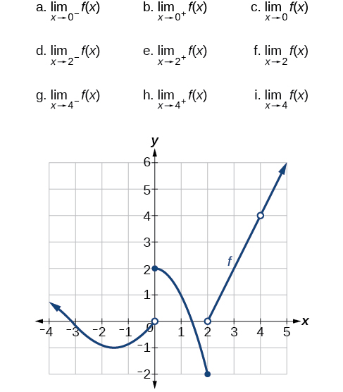
Using the graph of the function y=f(x) y=f(x) shown in Figure, estimate the following limits.
Solution
a. 0; b. 2; c. does not exist; d.−2; −2; e. 0; f. does not exist; g. 4; h. 4; i. 4
Finding a Limit Using a Table
Creating a table is a way to determine limits using numeric information. We create a table of values in which the input values of x approach a from both sides. Then we determine if the output values get closer and closer to some real value, the limit L.
Let’s consider an example using the following function:
limx→5(x3−125x−5)
To create the table, we evaluate the function at values close to x=5. We use some input values less than 5 and some values greater than 5 as in Figure. The table values show that when x>5 but nearing 5, the corresponding output gets close to 75. When x>5 but nearing 5, the corresponding output also gets close to 75.
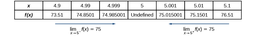
Because
limx→5−f(x)=75=limx→5+f(x),
then
limx→5f(x)=75.
Remember that f(5) does not exist.
How to: Given a function f,use a table to find the limit as x approaches a and the value of f(a), if it exists.
- Choose several input values that approach a a from both the left and right. Record them in a table.
- Evaluate the function at each input value. Record them in the table.
- Determine if the table values indicate a left-hand limit and a right-hand limit.
- If the left-hand and right-hand limits exist and are equal, there is a two-sided limit.
- Replace x with a to find the value of f(a).
Example 12.1.3: Finding a Limit Using a Table
Numerically estimate the limit of the following expression by setting up a table of values on both sides of the limit.
limx→0(5sin(x)3x)
Solution
We can estimate the value of a limit, if it exists, by evaluating the function at values near x=0. We cannot find a function value for x=0 directly because the result would have a denominator equal to 0, and thus would be undefined.
f(x)=5sin(x)3x
We create Figure by choosing several input values close to x=0, with half of them less than x=0 and half of them greater than x=0. Note that we need to be sure we are using radian mode. We evaluate the function at each input value to complete the table.
The table values indicate that when x<0 but approaching 0, the corresponding output nears 53.
When x>0 but approaching 0, the corresponding output also nears 53.

Because
limx→0−f(x)=53=limx→0+f(x),
then
limx→0f(x)=53.
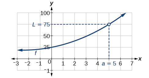
Q & A: Is it possible to check our answer using a graphing utility?
Yes. We previously used a table to find a limit of 75 for the function f(x)=x3−125x−5 as x approaches 5. To check, we graph the function on a viewing window as shown in Figure. A graphical check shows both branches of the graph of the function get close to the output 75 as x nears 5. Furthermore, we can use the ‘trace’ feature of a graphing calculator. By appraoching x=5 we may numerically observe the corresponding outputs getting close to 75.
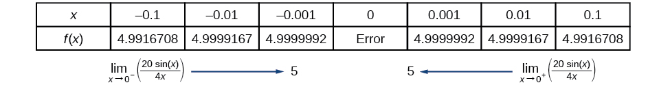
Exercise 12.1.3:
Numerically estimate the limit of the following function by making a table:
limx→0(20sin(x)4x)
Solution
limx→0(20sin(x)4x)=5
Q & A
Is one method for determining a limit better than the other?
No. Both methods have advantages. Graphing allows for quick inspection. Tables can be used when graphical utilities aren’t available, and they can be calculated to a higher precision than could be seen with an unaided eye inspecting a graph.
Example 12.1.4: Using a Graphing Utility to Determine a Limit
With the use of a graphing utility, if possible, determine the left- and right-hand limits of the following function as x approaches 0. If the function has a limit as x approaches 0, state it. If not, discuss why there is no limit.
f(x)=3 \sin (\dfrac{π}{x}) \nonumber
Solution
We can use a graphing utility to investigate the behavior of the graph close to x=0. Centering around x=0, we choose two viewing windows such that the second one is zoomed in closer to x=0 than the first one. The result would resemble Figure for [−2,2] by [−3,3].
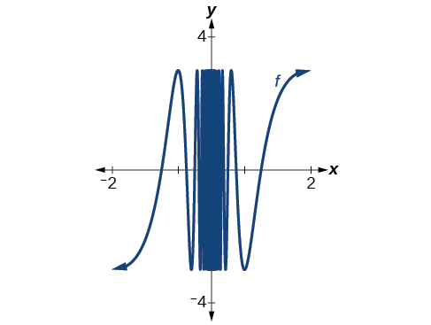
Even closer to zero, we are even less able to distinguish any limits.
The closer we get to 0, the greater the swings in the output values are. That is not the behavior of a function with either a left-hand limit or a right-hand limit. And if there is no left-hand limit or right-hand limit, there certainly is no limit to the function f(x) as x approaches 0.
We write
\lim_{x \to 0^−} \left( 3 \sin \left( \dfrac{π}{x} \right) \right) \;\;\; \text{does not exist.} \nonumber
\lim_{x \to 0^+} \left( 3 \sin \left( \dfrac{π}{x} \right) \right) \;\;\; \text{does not exist.} \nonumber
\lim_{x \to 0} \left( 3 \sin \left( \dfrac{π}{x} \right) \right) \;\;\; \text{does not exist.} \nonumber
Exercise \PageIndex{4}:
Numerically estimate the following limit: \lim \limits_{x \to 0} (\sin (\frac{2}{x})).
Solution
does not exist
Access these online resources for additional instruction and practice with finding limits.
Key Concepts
- A function has a limit if the output values approach some value L as the input values approach some quantity a. a. See Example.
- A shorthand notation is used to describe the limit of a function according to the form \lim \limits_{x \to a} f(x)=L, which indicates that as x approaches a, both from the left of x=a and the right of x=a, the output value gets close to L.
- A function has a left-hand limit if f(x) approaches L as x approaches a a where x<a. A function has a right-hand limit if f(x) approaches L as x approaches a where x>a.
- A two-sided limit exists if the left-hand limit and the right-hand limit of a function are the same. A function is said to have a limit if it has a two-sided limit.
- A graph provides a visual method of determining the limit of a function.
- If the function has a limit as x approaches a, the branches of the graph will approach the same y- coordinate near x=a from the left and the right. See Example.
- A table can be used to determine if a function has a limit. The table should show input values that approach a from both directions so that the resulting output values can be evaluated. If the output values approach some number, the function has a limit. See Example.
- A graphing utility can also be used to find a limit. See Example.
Footnotes
Glossary
- left-hand limit
- the limit of values of f(x) \nonumber as x approaches from a the left, denoted \lim \limits_{x \to a^−} f(x)=L. \nonumber The values of f(x) \nonumber can get as close to the limit L as we like by taking values of x sufficiently close to a a such that x<a \nonumber and x≠a. \nonumber . Both a and L are real numbers.
- limit
- when it exists, the value, L,that the output of a function f(x) approaches as the input x gets closer and closer to a but does not equal a. The value of the output, f(x), \nonumber can get as close to L as we choose to make it by using input values of x sufficiently near to x=a,but not necessarily at x=a. Both a and L are real numbers, and L is denoted \lim \limits_{x \to a}f(x)=L. \nonumber
- right-hand limit
- the limit of values of f(x) as x approaches a from the right, denoted \lim \limits_{x \to a^+}f(x)=L. \nonumber The values of f(x) can get as close to the limit L as we like by taking values of x sufficiently close to a where x>a, and x≠a. Both a and L are real numbers.
- two-sided limit
- the limit of a function f(x), \nonumber as x approaches a,is equal to L,that is, \lim \limits_{x \to a} f(x)=L \nonumber if and only if \lim \limits_{x \to a^−} f(x)= \lim \limits_{x \to a^+}f(x). \nonumber