8.3: Matrix Arithmetic

In Section 8.2, we used a special class of matrices, the augmented matrices, to assist us in solving systems of linear equations. In this section, we study matrices as mathematical objects of their own accord, temporarily divorced from systems of linear equations. To do so conveniently requires some more notation. When we write \(A = \left[ a_{ij} \right]_{m \times n}\), we mean \(A\) is an \(m\) by \(n\) matrix¹ and \(a_{ij}\) is the entry found in the \(i\)th row and \(j\)th column. Schematically, we have

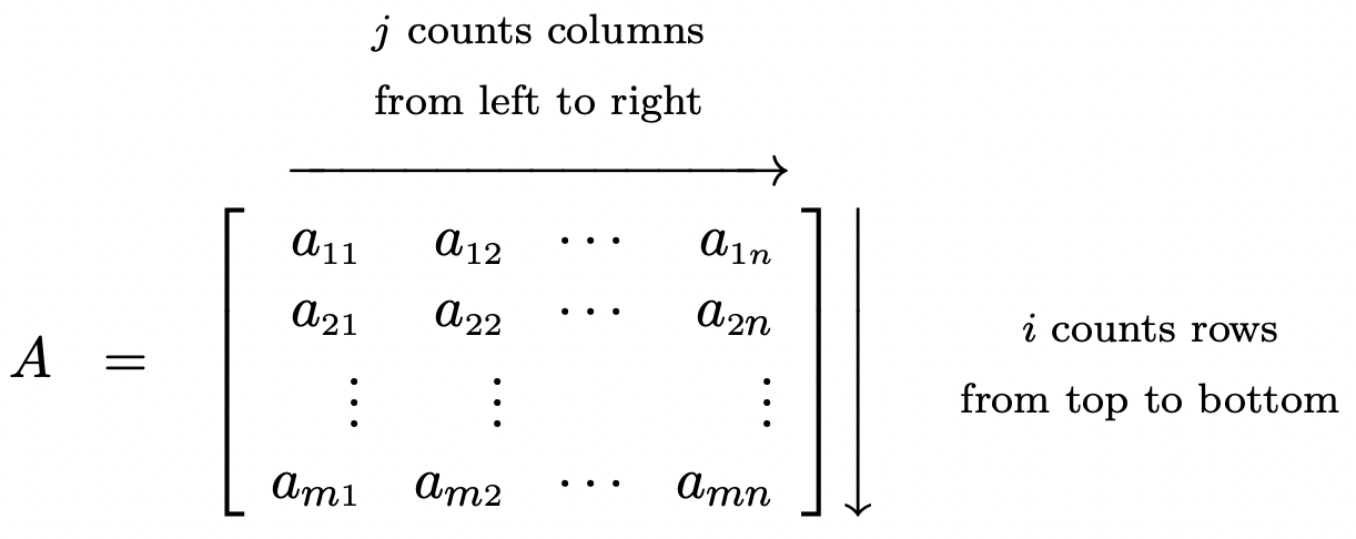
With this new notation we can define what it means for two matrices to be equal.

Definition 8.6.

Matrix Equality: Two matrices are said to be equal if they are the same size and their corresponding entries are equal. More specifically, if \(A =\left[a_{ij}\right]_{m \times n}\) and \(B =\left[b_{ij}\right]_{p \times r}\), we write \(A=B\) provided

1. \(m=p\) and \(n=r\)
2. \(a_{ij} = b_{ij}\) for all \(1 \leq i \leq m\) and all \(1 \leq j \leq n\).

Essentially, two matrices are equal if they are the same size and they have the same numbers in the same spots.² For example, the two \(2 \times 3\) matrices below are, despite appearances, equal.

\[\left[ \begin{array}{rrr} 0 & -2 & 9 \\ 25 & 117 & -3 \\ \end{array} \right] = \left[ \begin{array}{rrr} \ln(1) & \sqrt[3]{-8} & e^{2\ln(3)} \\ 125^{2/3} & 3^{2} \cdot 13 & \log(0.001) \end{array} \right]\nonumber\]

Now that we have an agreed upon understanding of what it means for two matrices to equal each other, we may begin defining arithmetic operations on matrices. Our first operation is addition.

Definition 8.7.

Matrix Addition: Given two matrices of the same size, the matrix obtained by adding the corresponding entries of the two matrices is called the sum of the two matrices. More specifically, if \(A =\left[a_{ij}\right]_{m \times n}\) and \(B =\left[b_{ij}\right]_{m \times n}\), we define \[A + B = \left[a_{ij}\right]_{m \times n} + \left[b_{ij}\right]_{m \times n} = \left[ a_{ij} + b_{ij} \right]_{m \times n}\nonumber\]

As an example, consider the sum below.

\[\left[ \begin{array}{rr}2 & 3 \\ 4 & -1 \\ 0 & -7 \\ \end{array} \right] + \left[ \begin{array}{rr} -1 & 4 \\ -5 & -3 \\ 8 & 1 \\ \end{array} \right] = \left[ \begin{array}{rr} 2 + (-1) & 3+4 \\ 4+(-5) & (-1)+(-3) \\ 0+8 & (-7)+ 1 \\ \end{array} \right] = \left[ \begin{array}{rr} 1 & 7 \\ -1 & -4 \\ 8 & -6 \\ \end{array} \right]\nonumber\]

It is worth the reader’s time to think what would have happened had we reversed the order of the summands above. As we would expect, we arrive at the same answer. In general, \(A+B = B+A\) for matrices \(A\) and \(B\), provided they are the same size so that the sum is defined in the first place. This is the commutative property of matrix addition. To see why this is true in general, we appeal to the definition of matrix addition. Given \(A =\left[a_{ij}\right]_{m \times n}\) and \(B =\left[b_{ij}\right]_{m \times n}\), \[A + B = \left[a_{ij}\right]_{m \times n} + \left[b_{ij}\right]_{m \times n} = \left[ a_{ij} + b_{ij} \right]_{m \times n} = \left[ b_{ij} + a_{ij} \right]_{m \times n} = \left[b_{ij}\right]_{m \times n} + \left[a_{ij}\right]_{m \times n} =B+A\nonumber\] where the second equality is the definition of \(A+B\), the third equality holds by the commutative law of real number addition, and the fourth equality is the definition of \(B+A\). In other words, matrix addition is commutative because real number addition is. A similar argument shows the associative property of matrix addition also holds, inherited in turn from the associative law of real number addition. Specifically, for matrices \(A\), \(B\), and \(C\) of the same size, \((A+B)+C = A+(B+C)\). In other words, when adding more than two matrices, it doesn’t matter how they are grouped. This means that we can write \(A+B+C\) without parentheses and there is no ambiguity as to what this means.³ These properties and more are summarized in the following theorem.

Theorem 8.3.

Properties of Matrix Addition

• Commutative Property: For all \(m \times n\) matrices, \(A + B = B + A\)
• Associative Property: For all \(m \times n\) matrices, \((A + B) + C = A + (B + C)\)
• Identity Property: If \(0_{m \times n}\) is the \(m \times n\) matrix whose entries are all \(0\), then \(0_{m \times n}\) is called the \(m \times n\) additive identity and for all \(m \times n\) matrices \(A\) \[A + 0_{m \times n} = 0_{m \times n} + A = A\nonumber\]
• Inverse Property: For every given \(m \times n\) matrix \(A\), there is a unique matrix denoted \(-A\) called the additive inverse of \(A\) such that \[A + (-A) = (-A) + A = 0_{m \times n}\nonumber\]

The identity property is easily verified by resorting to the definition of matrix addition; just as the number \(0\) is the additive identity for real numbers, the matrix comprised of all \(0\)’s does the same job for matrices. To establish the inverse property, given a matrix \(A=\left[a_{ij}\right]_{m \times n}\), we are looking for a matrix \(B = \left[b_{ij}\right]_{m \times n}\) so that \(A + B = 0_{m \times n}\). By the definition of matrix addition, we must have that \(a_{ij} + b_{ij} = 0\) for all \(i\) and \(j\). Solving, we get \(b_{ij} = -a_{ij}\). Hence, given a matrix \(A\), its additive inverse, which we call \(-A\), does exist and is unique and, moreover, is given by the formula: \(-A = \left[ - a_{ij}\right]_{m \times n}\). The long and short of this is: to get the additive inverse of a matrix, take additive inverses of each of its entries. With the concept of additive inverse well in hand, we may now discuss what is meant by subtracting matrices. You may remember from arithmetic that \(a - b = a+(-b)\); that is, subtraction is defined as ‘adding the opposite (inverse).’ We extend this concept to matrices. For two matrices \(A\) and \(B\) of the same size, we define \(A-B = A + (-B)\). At the level of entries, this amounts to

\[A-B = A + (-B) = \left[a_{ij}\right]_{m \times n} + \left[-b_{ij}\right]_{m \times n} = \left[a_{ij} + \left(-b_{ij}\right) \right]_{m \times n} = \left[a_{ij} - b_{ij} \right]_{m \times n}\nonumber\]

Thus to subtract two matrices of equal size, we subtract their corresponding entries. Surprised?

Our next task is to define what it means to multiply a matrix by a real number. Thinking back to arithmetic, you may recall that multiplication, at least by a natural number, can be thought of as ‘rapid addition.’ For example, \(2+2+2 = 3 \cdot 2\). We know from algebra⁴ that \(3x = x + x + x\), so it seems natural that given a matrix \(A\), we define \(3A = A + A + A\). If \(A =\left[a_{ij}\right]_{m \times n}\), we have \[3A = A + A + A = \left[a_{ij}\right]_{m \times n} + \left[a_{ij}\right]_{m \times n} + \left[a_{ij}\right]_{m \times n} = \left[a_{ij} + a_{ij} + a_{ij} \right]_{m \times n} = \left[ 3a_{ij}\right]_{m \times n}\nonumber\] In other words, multiplying the matrix in this fashion by \(3\) is the same as multiplying each entry by \(3\). This leads us to the following definition.

Definition 8.8.

Scalar^a Multiplication: We define the product of a real number and a matrix to be the matrix obtained by multiplying each of its entries by said real number. More specifically, if \(k\) is a real number and \(A = \left[a_{ij}\right]_{m \times n}\), we define \[kA = k\left[a_{ij}\right]_{m \times n} = \left[ka_{ij}\right]_{m \times n}\nonumber\]

---

^a The word ‘scalar’ here refers to real numbers. ‘Scalar multiplication’ in this context means we are multiplying a matrix by a real number (a scalar).

One may well wonder why the word ‘scalar’ is used for ‘real number.’ It has everything to do with ‘scaling’ factors.⁵ A point \(P(x,y)\) in the plane can be represented by its position matrix, \(P\):

\[(x,y) \leftrightarrow P = \left[ \begin{array}{r} x \\ y \\ \end{array} \right]\nonumber\]

Suppose we take the point \((-2,1)\) and multiply its position matrix by \(3\). We have\[3P = 3 \left[ \begin{array}{r} -2 \\ 1 \\ \end{array} \right] = \left[ \begin{array}{r} 3(-2) \\ 3(1) \\ \end{array} \right] = \left[ \begin{array}{r} -6 \\ 3 \\ \end{array} \right]\nonumber\] which corresponds to the point \((-6,3)\). We can imagine taking \((-2,1)\) to \((-6,3)\) in this fashion as a dilation by a factor of \(3\) in both the horizontal and vertical directions. Doing this to all points \((x,y)\) in the plane, therefore, has the effect of magnifying (scaling) the plane by a factor of \(3\).

As did matrix addition, scalar multiplication inherits many properties from real number arithmetic. Below we summarize these properties.

Theorem 8.4. Properties of Scalar Multiplication

• Associative Property: For every \(m \times n\) matrix \(A\) and scalars \(k\) and \(r\), \((kr)A = k(rA)\).
• Identity Property: For all \(m \times n\) matrices \(A\), \(1A = A\).
• Additive Inverse Property: For all \(m \times n\) matrices \(A\), \(-A = (-1)A\).
• Distributive Property of Scalar Multiplication over Scalar Addition: For every \(m \times n\) matrix \(A\) and scalars \(k\) and \(r\), \[(k+r)A = kA + rA\nonumber\]
• Distributive Property of Scalar Multiplication over Matrix Addition: For all \(m \times n\) matrices \(A\) and \(B\) scalars \(k\), \[k(A+B) = kA + kB\nonumber\]
• Zero Product Property: If \(A\) is an \(m \times n\) matrix and \(k\) is a scalar, then \[kA = 0_{m \times n} \quad \text{if and only if} \quad k=0 \quad \text{or} \quad A = 0_{m \times n}\nonumber\]

As with the other results in this section, Theorem 8.4 can be proved using the definitions of scalar multiplication and matrix addition. For example, to prove that \(k(A+B) = kA + kB\) for a scalar \(k\) and \(m \times n\) matrices \(A\) and \(B\), we start by adding \(A\) and \(B\), then multiplying by \(k\) and seeing how that compares with the sum of \(kA\) and \(kB\). \[k(A+B) = k \left(\left[a_{ij}\right]_{m \times n} + \left[b_{ij}\right]_{m \times n}\right) = k \left[a_{ij} + b_{ij} \right]_{m \times n} = \left[k \left(a_{ij}+b_{ij}\right)\right]_{m \times n} = \left[ka_{ij} + kb_{ij}\right]_{m \times n}\nonumber\]

As for \(kA + kB\), we have

\[kA + kB = k\left[a_{ij}\right]_{m \times n}+k\left[b_{ij}\right]_{m \times n} = \left[ka_{ij}\right]_{m \times n}+\left[kb_{ij}\right]_{m \times n} = \left[ka_{ij} + kb_{ij}\right]_{m \times n} \, \, \checkmark\nonumber\]

which establishes the property. The remaining properties are left to the reader. The properties in Theorems 8.3 and 8.4 establish an algebraic system that lets us treat matrices and scalars more or less as we would real numbers and variables, as the next example illustrates.

Example 8.3.1

Solve for the matrix \(A\): \(3A - \left(\left[ \begin{array}{rr} 2 & -1 \\ 3 & 5 \\ \end{array}\right] + 5A\right) = \left[ \begin{array}{rr} -4 & 2 \\ 6 & -2 \\ \end{array}\right] + \dfrac{1}{3} \left[ \begin{array}{rr} 9 & 12 \\ -3 & 39 \\ \end{array}\right]\) using the definitions and properties of matrix arithmetic.

Solution

\[\begin{array}{rcl} 3A - \left(\left[ \begin{array}{rr} 2 & -1 \\ 3 & 5 \\ \end{array}\right] + 5A\right) & = & \left[ \begin{array}{rr} -4 & 2 \\ 6 & -2 \\ \end{array}\right] + \dfrac{1}{3} \left[ \begin{array}{rr} 9 & 12 \\ -3 & 39 \\ \end{array}\right] \\ 3A + \left\{-\left(\left[ \begin{array}{rr} 2 & -1 \\ 3 & 5 \\ \end{array}\right] + 5A \right)\right\} & = & \left[ \begin{array}{rr} -4 & 2 \\ 6 & -2 \\ \end{array}\right] + \left[ \begin{array}{rr} \left(\frac{1}{3}\right)(9) & \left(\frac{1}{3}\right)(12) \\[2pt] \left(\frac{1}{3}\right)(-3) & \left(\frac{1}{3}\right)(39) \\ \end{array}\right] \\ 3A + (-1)\left(\left[ \begin{array}{rr} 2 & -1 \\ 3 & 5 \\ \end{array}\right] + 5A \right) & = & \left[ \begin{array}{rr} -4 & 2 \\ 6 & -2 \\ \end{array}\right] + \left[ \begin{array}{rr} 3 & 4 \\ -1 & 13 \\ \end{array}\right] \\ 3A + \left\{ (-1)\left[ \begin{array}{rr} 2 & -1 \\ 3 & 5 \\ \end{array}\right] + (-1)(5A)\right \} & = & \left[ \begin{array}{rr} -1 & 6 \\ 5 & 11 \\ \end{array}\right] \\ 3A + (-1)\left[ \begin{array}{rr} 2 & -1 \\ 3 & 5 \\ \end{array}\right] + (-1)(5A) & = & \left[ \begin{array}{rr} -1 & 6 \\ 5 & 11 \\ \end{array}\right] \\ 3A + \left[ \begin{array}{rr} (-1)(2) & (-1)(-1) \\ (-1)(3) & (-1)(5) \\ \end{array}\right] + ((-1)(5))A & = & \left[ \begin{array}{rr} -1 & 6 \\ 5 & 11 \\ \end{array}\right] \\ 3A + \left[ \begin{array}{rr} -2 & 1 \\ -3 & -5 \\ \end{array}\right] + (-5)A & = & \left[ \begin{array}{rr} -1 & 6 \\ 5 & 11 \\ \end{array}\right] \\ 3A + (-5)A+ \left[ \begin{array}{rr} -2 & 1 \\ -3 & -5 \\ \end{array}\right]& = & \left[ \begin{array}{rr} -1 & 6 \\ 5 & 11 \\ \end{array}\right] \\ (3+ (-5))A+ \left[ \begin{array}{rr} -2 & 1 \\ -3 & -5 \\ \end{array}\right] + \left(-\left[ \begin{array}{rr} -2 & 1 \\ -3 & -5 \\ \end{array}\right] \right)& = & \left[ \begin{array}{rr} -1 & 6 \\ 5 & 11 \\ \end{array}\right] + \left(-\left[ \begin{array}{rr} -2 & 1 \\ -3 & -5 \\ \end{array}\right] \right) \\ (-2)A+ 0_{2 \times 2} & = & \left[ \begin{array}{rr} -1 & 6 \\ 5 & 11 \\ \end{array}\right] -\left[ \begin{array}{rr} -2 & 1 \\ -3 & -5 \\ \end{array}\right] \\ (-2)A & = & \left[ \begin{array}{rr} -1 - (-2) & 6 - 1 \\ 5 - (-3) & 11 - (-5) \\ \end{array}\right] \\ (-2)A & = & \left[ \begin{array}{rr} 1 & 5 \\ 8 & 16 \\ \end{array}\right] \\ \left(-\frac{1}{2}\right)\left((-2)A\right) & = & -\frac{1}{2} \left[ \begin{array}{rr} 1 & 5 \\ 8 & 16 \\ \end{array}\right] \\ \left(\left(-\frac{1}{2}\right)(-2)\right)A & = & \left[ \begin{array}{rr} \left(-\frac{1}{2}\right)(1) & \left(-\frac{1}{2}\right)(5) \\[2pt] \left(-\frac{1}{2}\right)(8) & \left(-\frac{1}{2}\right)(16) \\ \end{array}\right] \\ 1 A & = & \left[ \begin{array}{rr} -\frac{1}{2} & -\frac{5}{2} \\[2pt] -4 & -\frac{16}{2} \\ \end{array}\right] \\ A & = & \left[ \begin{array}{rr} -\frac{1}{2} & -\frac{5}{2} \\[2pt] -4 & -8 \\ \end{array}\right] \\ \end{array}\nonumber\] The reader is encouraged to check our answer in the original equation.

While the solution to the previous example is written in excruciating detail, in practice many of the steps above are omitted. We have spelled out each step in this example to encourage the reader to justify each step using the definitions and properties we have established thus far for matrix arithmetic. The reader is encouraged to solve the equation in Example 8.3.1 as they would any other linear equation, for example: \(3a-(2+5a)=-4+\frac{1}{3}(9)\).

We now turn our attention to matrix multiplication - that is, multiplying a matrix by another matrix. Based on the ‘no surprises’ trend so far in the section, you may expect that in order to multiply two matrices, they must be of the same size and you find the product by multiplying the corresponding entries. While this kind of product is used in other areas of mathematics,⁶ we define matrix multiplication to serve us in solving systems of linear equations. To that end, we begin by defining the product of a row and a column. We motivate the general definition with an example. Consider the two matrices \(A\) and \(B\) below.

\[\begin{array}{cc} A = \left[\begin{array}{rrr} 2 & \hphantom{-}0 & -1 \\ -10 & 3 & 5 \\ \end{array} \right] & B = \left[\begin{array}{rrrr} 3 & \hphantom{-}1 & 2 & -8 \\ 4 & 8 & -5 & 9 \\ 5 & 0 & -2 & -12 \\ \end{array} \right] \end{array}\nonumber\]

Let \(R1\) denote the first row of \(A\) and \(C1\) denote the first column of \(B\). To find the ‘product’ of \(R1\) with \(C1\), denoted \(R1 \cdot C1\), we first find the product of the first entry in \(R1\) and the first entry in \(C1\). Next, we add to that the product of the second entry in \(R1\) and the second entry in \(C1\). Finally, we take that sum and we add to that the product of the last entry in \(R1\) and the last entry in \(C1\). Using entry notation, \(R1 \cdot C1 = a_{11}b_{11} + a_{12}b_{21}+a_{13}b_{31} = (2)(3) + (0)(4) + (-1)(5) = 6 + 0 + (-5) = 1\). We can visualize this schematically as follows

\[\left[\begin{array}{rrr} \rowcolor[gray]{0.9} 2 & \hphantom{-}0 & -1 \\ -10 & 3 & 5 \\ \end{array} \right] \left[\begin{array}{>{\columncolor[gray]{0.9}}rrrr} 3 & \hphantom{-}1 & 2 & -8 \\ 4 & 8 & -5 & 9 \\ 5 & 0 & -2 & -12 \\ \end{array} \right]\nonumber\]

\[\begin{array}{ccccc} \underbrace{\begin{array}{rl} \stackrel{\xrightarrow{\hspace{.75in}}}{\begin{array}{ccc} \fbox{2} & \hphantom{-}0 & -1 \end{array}} & \left. \begin{array}{c} \fbox{3} \\ 4 \\ 5 \\ \end{array} \right\downarrow \\ \end{array}} & & \underbrace{\begin{array}{rl} \stackrel{\xrightarrow{\hspace{.75in}}}{\begin{array}{ccc} 2 & \hphantom{-}\fbox{0} & -1 \end{array}} & \left. \begin{array}{c} 3 \\ \fbox{4} \\ 5 \\ \end{array} \right\downarrow \\\end{array}} & & \underbrace{\begin{array}{rl} \stackrel{\xrightarrow{\hspace{.75in}}}{\begin{array}{ccc} 2 & \hphantom{-}0 & \fbox{$-1$} \end{array}} & \left. \begin{array}{c} 3 \\ 4 \\ \fbox{5} \\ \end{array} \right\downarrow \\ \end{array}} \\ a_11b_11 & + & a_12b_21 & + & a_13b_31 \\ (2)(3) & + &(0)(4)& + & (-1)(5) \\ \end{array}\nonumber\]

To find \(R2 \cdot C3\) where \(R2\) denotes the second row of \(A\) and \(C3\) denotes the third column of \(B\), we proceed similarly. We start with finding the product of the first entry of \(R2\) with the first entry in \(C3\) then add to it the product of the second entry in \(R2\) with the second entry in \(C3\), and so forth. Using entry notation, we have \(R2 \cdot C3 = a_{21}b_{13} + a_{22}b_{23} + a_{23}b_{33} = (-10)(2) + (3)(-5) + (5)(-2) = -45\). Schematically,

\[\left[\begin{array}{rrr} 2 & 0 & -1 \\ \rowcolor[gray]{0.9} -10 & \hphantom{-}3 & 5 \\ \end{array} \right] \left[\begin{array}{rr>{\columncolor[gray]{0.9}}rr} 3 & \hphantom{-}1 & 2 & -8 \\ 4 & 8 & -5 & 9 \\ 5 & 0 & -2 & -12 \\ \end{array} \right]\nonumber\]

\[\begin{array}{ccccc} \underbrace{\begin{array}{rl} \stackrel{\xrightarrow{\hspace{.75in}}}{\begin{array}{ccc} \fbox{$-10$} & 3 & 5 \end{array}} & \left. \begin{array}{c} \fbox{\hphantom{$-$}2} \\ -5 \\ -2 \\ \end{array} \right\downarrow \\ \end{array}} & & \underbrace{\begin{array}{rl} \stackrel{\xrightarrow{\hspace{.75in}}}{\begin{array}{ccc} -10 & \fbox{3} & 5 \end{array}} & \left. \begin{array}{c} \hphantom{-}2 \\ \fbox{$-5$} \\ -2 \\ \end{array} \right\downarrow \\\end{array}} & & \underbrace{\begin{array}{rl} \stackrel{\xrightarrow{\hspace{.75in}}}{\begin{array}{ccc} -10 & 3 & \fbox{$5$} \end{array}} & \left. \begin{array}{c} \hphantom{-}2 \\ -5 \\ \fbox{$-2$} \\ \end{array} \right\downarrow \\ \end{array}} \\ a_21b_13= (-10)(2) = -20 & + & a_22b_23 = (3)(-5) = -15 & + & a_23b_33 = (5)(-2) = -10 \\ \end{array}\nonumber\]

Generalizing this process, we have the following definition.

Definition 8.9.

Product of a Row and a Column: Suppose \(A = [a_{ij}]_{m \times n}\) and \(B = [b_{ij}]_{n \times r}\). Let \(Ri\) denote the \(i\)th row of \(A\) and let \(Cj\) denote the \(j\)th column of \(B\). The product of \(R_{i}\) and \(C_{j}\), denoted \(R_{i} \cdot C_{j}\) is the real number defined by \[Ri \cdot Cj = a_{i\mbox{\tiny$1$}}b_1$}j} + a_{i\mbox{\tiny$2b_{\mbox{\tiny$2$}j} + \ldots a_{in}b_{nj}\nonumber\]

Note that in order to multiply a row by a column, the number of entries in the row must match the number of entries in the column. We are now in the position to define matrix multiplication.

Definition 8.10.

Matrix Multiplication: Suppose \(A = [a_{ij}]_{m \times n}\) and \(B = [b_{ij}]_{n \times r}\). Let \(Ri\) denote the \(i\)th row of \(A\) and let \(Cj\) denote the \(j\)th column of \(B\). The product of \(A\) and \(B\), denoted \(AB\), is the matrix defined by \[AB = \left[ Ri \cdot Cj \right]_{m \times r}\nonumber\]

that is

\[AB = \left[ \begin{array}{cccc} R1 \cdot C1 & R1 \cdot C2 & \ldots & R1 \cdot Cr \\ R2 \cdot C1 & R2 \cdot C2 & \ldots & R2 \cdot Cr \\ \vdots & \vdots & & \vdots \\ Rm \cdot C1 & Rm \cdot C2 & \ldots & Rm \cdot Cr \\ \end{array} \right]\nonumber\]

There are a number of subtleties in Definition 8.10 which warrant closer inspection. First and foremost, Definition 8.10 tells us that the \(ij\)-entry of a matrix product \(AB\) is the \(i\)th row of \(A\) times the \(j\)th column of \(B\). In order for this to be defined, the number of entries in the rows of \(A\) must match the number of entries in the columns of \(B\). This means that the number of columns of \(A\) must match⁷ the number of rows of \(B\). In other words, to multiply \(A\) times \(B\), the second dimension of \(A\) must match the first dimension of \(B\), which is why in Definition 8.10, \(A_{m \times \underline{n}}\) is being multiplied by a matrix \(B_{\underline{n} \times r}\). Furthermore, the product matrix \(AB\) has as many rows as \(A\) and as many columns of \(B\). As a result, when multiplying a matrix \(A_{\underline{m} \times n}\) by a matrix \(B_{n \times \underline{r}}\), the result is the matrix \(AB_{\underline{m} \times \underline{r}}\). Returning to our example matrices below, we see that \(A\) is a \(2 \times \underline{3}\) matrix and \(B\) is a \(\underline{3} \times 4\) matrix. This means that the product matrix \(AB\) is defined and will be a \(2 \times 4\) matrix.

\[\begin{array}{cc} A = \left[\begin{array}{rrr} 2 & \hphantom{-}0 & -1 \\ -10 & 3 & 5 \\ \end{array} \right] & B = \left[\begin{array}{rrrr} 3 & \hphantom{-}1 & 2 & -8 \\ 4 & 8 & -5 & 9 \\ 5 & 0 & -2 & -12 \\ \end{array} \right] \end{array}\nonumber\]

Using \(Ri\) to denote the \(i\)th row of \(A\) and \(Cj\) to denote the \(j\)th column of \(B\), we form \(AB\) according to Definition 8.10.

\[\begin{array}{rclcl} AB & = & \left[\begin{array}{rrrr} R1 \cdot C1 & R1 \cdot C2 & R1 \cdot C3 & R1 \cdot C4 \\ R2 \cdot C1 & R2 \cdot C2 & R2 \cdot C3 & R2 \cdot C4 \\ \end{array} \right] & = & \left[\begin{array}{rrrr} 1 & \hphantom{-}2 & 6 & -4 \\ 7 & 14 & -45 & 47 \\ \end{array} \right] \\ \end{array}\nonumber\]

Note that the product \(BA\) is not defined, since \(B\) is a \(3 \times \underline{4}\) matrix while \(A\) is a \(\underline{2} \times 3\) matrix; \(B\) has more columns than \(A\) has rows, and so it is not possible to multiply a row of \(B\) by a column of \(A\). Even when the dimensions of \(A\) and \(B\) are compatible such that \(AB\) and \(BA\) are both defined, the product \(AB\) and \(BA\) aren’t necessarily equal.⁸ In other words, \(AB\) may not equal \(BA\). Although there is no commutative property of matrix multiplication in general, several other real number properties are inherited by matrix multiplication, as illustrated in our next theorem.

Theorem 8.5

Properties of Matrix Multiplication Let \(A\), \(B\) and \(C\) be matrices such that all of the matrix products below are defined and let \(k\) be a real number.

• Associative Property of Matrix Multiplication: \((AB)C = A(BC)\)
• Associative Property with Scalar Multiplication: \(k(AB) = (kA)B = A(kB)\)
• Identity Property: For a natural number \(k\), the \(k \times k\) identity matrix, denoted \(I_{k}\), is defined by \(I_{k} = \left[d_{ij} \right]_{k \times k}\) where\[d_{ij} = \left\{ \begin{array}{rl} 1, & \text{if $i=j$} \\ 0, & \text{otherwise} \\ \end{array} \right.\nonumber\]For all \(m \times n\) matrices, \(I_{m}A = AI_{n} = A\).
• Distributive Property of Matrix Multiplication over Matrix Addition: \[A(B \pm C) = AB \pm AC \mbox{ and } (A \pm B)C = AC \pm BC\nonumber\]

The one property in Theorem 8.5 which begs further investigation is, without doubt, the multiplicative identity. [maindiagonal] The entries in a matrix where \(i=j\) comprise what is called the main diagonal of the matrix. The identity matrix has \(1\)’s along its main diagonal and \(0\)’s everywhere else. A few examples of the matrix \(I_{k}\) mentioned in Theorem 8.5 are given below. The reader is encouraged to see how they match the definition of the identity matrix presented there.

\[\begin{array}{ccccc} [1] & \left[ \begin{array}{rr} 1 & 0 \\ 0 & 1 \\ \end{array} \right] & \left[ \begin{array}{rrr} 1 & 0 & 0 \\ 0 & 1 & 0 \\ 0 & 0 & 1 \\ \end{array} \right] & \left[ \begin{array}{rrrr} 1 & 0 & 0 & 0 \\ 0 & 1 & 0 & 0 \\ 0 & 0 & 1 & 0 \\ 0 & 0 & 0 & 1 \\ \end{array} \right] \\ I_1 & I_2 & I_3 & I_4 \\ \end{array}\nonumber\]

The identity matrix is an example of what is called a square matrix as it has the same number of rows as columns. Note that to in order to verify that the identity matrix acts as a multiplicative identity, some care must be taken depending on the order of the multiplication. For example, take the matrix \(2 \times 3\) matrix \(A\) from earlier

\[A = \left[\begin{array}{rrr} 2 & \hphantom{-}0 & -1 \\ -10 & 3 & 5 \\ \end{array} \right]\nonumber\]

In order for the product \(I_{k}A\) to be defined, \(k = 2\); similarly, for \(AI_{k}\) to be defined, \(k = 3\). We leave it to the reader to show \(I_{2}A = A\) and \(AI_{3} = A\). In other words,

\[\begin{array}{rcl} \left[ \begin{array}{rr} 1 & 0 \\ 0 & 1 \\ \end{array} \right] \left[\begin{array}{rrr} 2 & \hphantom{-}0 & -1 \\ -10 & 3 & 5 \\ \end{array} \right] & = & \left[\begin{array}{rrr} 2 & \hphantom{-}0 & -1 \\ -10 & 3 & 5 \\ \end{array} \right] \\ \end{array}\nonumber\]

and \[\begin{array}{rcl} \left[\begin{array}{rrr} 2 & \hphantom{-}0 & -1 \\ -10 & 3 & 5 \\ \end{array} \right]\left[ \begin{array}{rrr} 1 & 0 & 0 \\ 0 & 1 & 0 \\ 0 & 0 & 1 \\ \end{array} \right] & = & \left[\begin{array}{rrr} 2 & \hphantom{-}0 & -1 \\ -10 & 3 & 5 \\ \end{array} \right] \\ \end{array}\nonumber\]

While the proofs of the properties in Theorem 8.5 are computational in nature, the notation becomes quite involved very quickly, so they are left to a course in Linear Algebra. The following example provides some practice with matrix multiplication and its properties. As usual, some valuable lessons are to be learned.

Example 8.3.2

1. Find \(AB\) for \(A = \left[ \begin{array}{rrr} -23 & -1 & 17 \\ 46 & 2 & -34 \\ \end{array} \right]\) and \(B = \left[ \begin{array}{rr} -3 & 2 \\ 1 & 5 \\ -4 & 3 \\ \end{array} \right]\)
2. Find \(C^2 -5C + 10I_{2}\) for \(C = \left[ \begin{array}{rr} 1 & -2 \\ 3 & 4 \\ \end{array} \right]\)
3. Suppose \(M\) is a \(4 \times 4\) matrix. Use Theorem 8.5 to expand \(\left(M - 2I_{4}\right)\left(M + 3I_{4}\right)\).

Solution.

1. We have \(AB = \left[ \begin{array}{rrr} -23 & -1 & 17 \\ 46 & 2 & -34 \end{array} \right] \left[ \begin{array}{rr} -3 & 2 \\ 1 & 5 \\ -4 & 3 \end{array} \right] = \left[ \begin{array}{rr} 0 & 0 \\ 0 & 0 \end{array} \right]\)
2. Just as \(x^2\) means \(x\) times itself, \(C^2\) denotes the matrix \(C\) times itself. We get

   \[\begin{array}{rcl} C^2 -5C + 10I_2 & = & \left[ \begin{array}{rr} 1 & -2 \\ 3 & 4 \\ \end{array} \right]^2 - 5 \left[ \begin{array}{rr} 1 & -2 \\ 3 & 4 \\ \end{array} \right] + 10 \left[ \begin{array}{rr} 1 & 0 \\ 0 & 1 \\ \end{array} \right] \\ & = & \left[ \begin{array}{rr} 1 & -2 \\ 3 & 4 \\ \end{array} \right]\left[ \begin{array}{rr} 1 & -2 \\ 3 & 4 \\ \end{array} \right] + \left[ \begin{array}{rr} -5 & 10 \\ -15 & -20 \\ \end{array} \right] + \left[ \begin{array}{rr} 10 & 0 \\ 0 & 10 \\ \end{array} \right] \\ & = & \left[ \begin{array}{rr} -5 & -10 \\ 15 & 10 \\ \end{array} \right] + \left[ \begin{array}{rr} 5 & 10 \\ -15 & -10 \\ \end{array} \right] \\ & = & \left[ \begin{array}{rr} 0 & 0 \\ 0 & 0 \\ \end{array} \right] \\ \end{array}\nonumber\]

3. We expand \(\left(M - 2I_{4}\right)\left(M + 3I_{4}\right)\) with the same pedantic zeal we showed in Example 8.3.1. The reader is encouraged to determine which property of matrix arithmetic is used as we proceed from one step to the next.

   \[\begin{array}{rcl} \left(M - 2I_4\right)\left(M + 3I_4\right) & = & \left(M - 2I_4\right) M + \left(M - 2I_4\right)\left( 3I_4\right) \\ & = & MM - \left(2I_4\right)M + M\left( 3I_4\right) - \left( 2I_4\right)\left( 3I_4\right) \\ & = & M^2 -2 \left(I_4M\right) +3\left( M I_4\right) - 2\left( I_4\left( 3I_4\right)\right) \\ & = & M^2 - 2M + 3M - 2\left(3\left( I_4I_4\right)\right) \\ & = & M^2 +M - 6I_4 \\ \end{array}\nonumber\]

1. Example 8.3.2 illustrates some interesting features of matrix multiplication. First note that in part 1, neither \(A\) nor \(B\) is the zero matrix, yet the product \(AB\) is the zero matrix. Hence, the the zero product property enjoyed by real numbers and scalar multiplication does not hold for matrix multiplication. Parts 2 and 3 introduce us to polynomials involving matrices. The reader is encouraged to step back and compare our expansion of the matrix product \(\left(M - 2I_{4}\right)\left(M + 3I_{4}\right)\) in part 3 with the product \((x-2)(x+3)\) from real number algebra. The exercises explore this kind of parallel further.

As we mentioned earlier, a point \(P(x,y)\) in the \(xy\)-plane can be represented as a \(2 \times 1\) position matrix. We now show that matrix multiplication can be used to rotate these points, and hence graphs of equations.

Example 8.3.3

Let \(R = \left[ \begin{array}{rr} \frac{\sqrt{2}}{2} & -\frac{\sqrt{2}}{2} \\[4pt] \frac{\sqrt{2}}{2} & \frac{\sqrt{2}}{2} \end{array} \right]\).

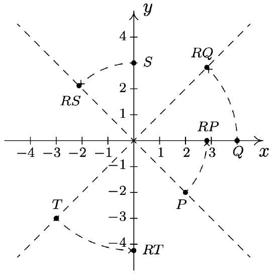
1. Plot \(P(2,-2)\), \(Q(4,0)\), \(S(0,3)\), and \(T(-3,-3)\) in the plane as well as the points \(RP\), \(RQ\), \(RS\), and \(RT\). Plot the lines \(y=x\) and \(y=-x\) as guides. What does \(R\) appear to be doing to these points?
2. If a point \(P\) is on the hyperbola \(x^2-y^2=4\), show that the point \(RP\) is on the curve \(y = \frac{2}{x}\).

Solution

For \(P(2,-2)\), the position matrix is \(P = \left[ \begin{array}{r} 2 \\ -2 \\ \end{array} \right]\), and

\[\begin{array}{rcl} RP & = & \left[ \begin{array}{rr} \frac{\sqrt{2}}{2} & -\frac{\sqrt{2}}{2} \\[4pt] \frac{\sqrt{2}}{2} & \frac{\sqrt{2}}{2} \\ \end{array} \right]\left[ \begin{array}{r} 2 \\[4pt] -2 \\ \end{array} \right] \\ & = & \left[ \begin{array}{r} 2\sqrt{2} \\ 0 \\ \end{array} \right] \\ \end{array}\nonumber\]

We have that \(R\) takes \((2,-2)\) to \((2 \sqrt{2}, 0)\). Similarly, we find \((4,0)\) is moved to \((2\sqrt{2}, 2\sqrt{2})\), \((0,3)\) is moved to \(\left(-\frac{3 \sqrt{2}}{2}, \frac{3 \sqrt{2}}{2} \right)\), and \((-3,-3)\) is moved to \((0,-3\sqrt{2})\). Plotting these in the coordinate plane along with the lines \(y=x\) and \(y=-x\), we see that the matrix \(R\) is rotating these points counterclockwise by \(45^{\circ}\).

For a generic point \(P(x,y)\) on the hyperbola \(x^2-y^2=4\), we have

\[\begin{array}{rcl} RP & = & \left[ \begin{array}{rr} \frac{\sqrt{2}}{2} & -\frac{\sqrt{2}}{2} \\[4pt] \frac{\sqrt{2}}{2} & \frac{\sqrt{2}}{2} \\ \end{array} \right]\left[ \begin{array}{r} x \\[4pt] y \\ \end{array} \right] \\ & = & \left[ \begin{array}{r} \frac{\sqrt{2}}{2} x - \frac{\sqrt{2}}{2} y \\[4pt] \frac{\sqrt{2}}{2} x + \frac{\sqrt{2}}{2} y \\ \end{array} \right] \\ \end{array}\nonumber\]

which means \(R\) takes \((x,y)\) to \(\left(\frac{\sqrt{2}}{2} x - \frac{\sqrt{2}}{2} y, \frac{\sqrt{2}}{2} x + \frac{\sqrt{2}}{2} y\right)\). To show that this point is on the curve \(y = \frac{2}{x}\), we replace \(x\) with \(\frac{\sqrt{2}}{2} x - \frac{\sqrt{2}}{2} y\) and \(y\) with \(\frac{\sqrt{2}}{2} x + \frac{\sqrt{2}}{2} y\) and simplify.

\[\begin{array}{rcl} y & = & \frac{2}{x} \\ \frac{\sqrt{2}}{2} x + \frac{\sqrt{2}}{2} y & \stackrel{?}{=} & \frac{2}{\frac{\sqrt{2}}{2} x - \frac{\sqrt{2}}{2} y} \\[10pt] \left(\frac{\sqrt{2}}{2} x - \frac{\sqrt{2}}{2} y \right) \left(\frac{\sqrt{2}}{2} x + \frac{\sqrt{2}}{2} y \right)& \stackrel{?}{=} & \left(\dfrac{2}{\frac{\sqrt{2}}{2} x - \frac{\sqrt{2}}{2} y}\right) \left( \frac{\sqrt{2}}{2} x - \frac{\sqrt{2}}{2} y \right)\\ \left(\frac{\sqrt{2}}{2} x \right)^2 - \left( \frac{\sqrt{2}}{2} y\right)^2 & \stackrel{?}{=} & 2 \\ \frac{x^2}{2} - \frac{y^2}{2} & \stackrel{?}{=} & 2 \\ x^2 - y^2 & \stackrel{\checkmark }{=}& 4 \\ \end{array}\nonumber\]

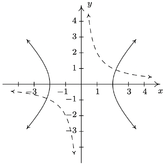
Since \((x,y)\) is on the hyperbola \(x^2 - y^2 = 4\), we know that this last equation is true. Since all of our steps are reversible, this last equation is equivalent to our original equation, which establishes the point is, indeed, on the graph of \(y = \frac{2}{x}\). This means the graph of \(y=\frac{2}{x}\) is a hyperbola, and it is none other than the hyperbola \(x^2-y^2=4\) rotated counterclockwise by \(45^{\circ}\).⁹ Below we have the graph of \(x^2-y^2=4\) (solid line) and \(y = \frac{2}{x}\) (dashed line) for comparison.

When we started this section, we mentioned that we would temporarily consider matrices as their own entities, but that the algebra developed here would ultimately allow us to solve systems of linear equations. To that end, consider the system

\[\left\{ \begin{array}{rcl} 3x - y + z & = & 8 \\ x + 2y - z & = & 4 \\ 2x+ 3y - 4z & = & 10 \\ \end{array} \right.\nonumber\]

In Section 8.2, we encoded this system into the augmented matrix

\[\left[ \begin{array}{rrr|r} 3 & -1 & 1 & 8 \\ 1 & 2 & -1 & 4 \\ 2 & 3 & -4 & 10 \\ \end{array} \right]\nonumber\]

Recall that the entries to the left of the vertical line come from the coefficients of the variables in the system, while those on the right comprise the associated constants. For that reason, we may form the coefficient matrix \(A\), the unknowns matrix \(X\) and the constant matrix \(B\) as below

\[\begin{array}{ccc} A = \left[ \begin{array}{rrr} 3 & -1 & 1 \\ 1 & 2 & -1 \\ 2 & 3 & -4 \\ \end{array} \right] & X = \left[ \begin{array}{r} x \\ y \\ z \\ \end{array} \right] & B = \left[ \begin{array}{r} 8 \\ 4 \\ 10 \\ \end{array} \right] \end{array}\nonumber\]

We now consider the matrix equation \(AX = B\).

\[\begin{array}{rcl} AX & = & B \\ \left[ \begin{array}{rrr} 3 & -1 & 1 \\ 1 & 2 & -1 \\ 2 & 3 & -4 \\ \end{array} \right] \left[ \begin{array}{r} x \\ y \\ z \\ \end{array} \right] & = & \left[ \begin{array}{r} 8 \\ 4 \\ 10 \\ \end{array} \right] \\ \left[ \begin{array}{rrr} 3x -y +z \\ x + 2y -z \\ 2x + 3y -4 z \\ \end{array} \right] & = & \left[ \begin{array}{r} 8 \\ 4 \\ 10 \\ \end{array} \right] \\ \end{array}\nonumber\]

We see that finding a solution \((x,y,z)\) to the original system corresponds to finding a solution \(X\) for the matrix equation \(AX = B\). If we think about solving the real number equation \(ax = b\), we would simply ‘divide’ both sides by \(a\). Is it possible to ‘divide’ both sides of the matrix equation \(AX = B\) by the matrix \(A\)? This is the central topic of Section 8.4.

8.3.1. Exercises

For each pair of matrices \(A\) and \(B\) in Exercises 1 - 7, find the following, if defined

• \(3A\)
• \(-B\)
• \(A^2\)
• \(A-2B\)
• \(AB\)
• \(BA\)

1. \(A = \left[ \begin{array}{rr} 2 & -3 \\ 1 & 4 \end{array} \right]\), \(B=\left[ \begin{array}{rr} 5 & -2 \\ 4 & 8 \end{array} \right]\)
2. \(A = \left[ \begin{array}{rr} -1 & 5 \\ -3 & 6 \end{array} \right]\), \(B=\left[ \begin{array}{rr} 2 & 10 \\ -7 & 1 \end{array} \right]\)
3. \(A = \left[ \begin{array}{rr} -1 & 3 \\ 5 & 2 \end{array} \right]\), \(B=\left[ \begin{array}{rrr} 7 & 0 & 8 \\ -3 & 1 & 4 \end{array} \right]\)
4. \(A = \left[ \begin{array}{rr} 2 & 4 \\ 6 & 8 \end{array} \right]\), \(B=\left[ \begin{array}{rrr} -1 & 3 & -5 \\ 7 & -9 & 11 \end{array} \right]\)
5. \(A = \left[ \begin{array}{r} 7 \\ 8 \\ 9 \end{array} \right]\), \(B=\left[ \begin{array}{rrr} 1 & 2 & 3 \end{array} \right]\)
6. \(A = \left[ \begin{array}{rr} 1 & -2 \\ -3 & 4 \\ 5 & -6 \end{array} \right]\), \(B=\left[ \begin{array}{rrr} -5 & 1 & 8 \end{array} \right]\)
7. \(A = \left[ \begin{array}{rrr} 2 & -3 & 5 \\ 3 & 1 &-2 \\ -7 & 1 & -1 \end{array} \right]\), \(B= \left[ \begin{array}{rrr} 1 & 2 & 1 \\ 17 & 33 & 19 \\ 10 & 19 & 11 \end{array} \right]\)

In Exercises 8 - 21, use the matrices \[A = \left[ \begin{array}{rr} 1 & 2 \\ 3 & 4 \end{array} \right] \;\;\; B = \left[ \begin{array}{rr} 0 & -3 \\ -5 & 2 \end{array} \right] \;\;\; C = \left[ \begin{array}{rrr} 10 & -\frac{11}{2} & 0 \\ \frac{3}{5} & 5 & 9 \end{array} \right]\nonumber\] \[D = \left[ \begin{array}{rr} 7 & -13 \\ -\frac{4}{3} & 0 \\ 6 & 8 \end{array} \right] \;\;\; E = \left[ \begin{array}{rrr} 1 & \hphantom{-}2 & 3 \\ 0 & 4 & -9 \\ 0 & 0 & -5 \end{array} \right]\nonumber\] to compute the following or state that the indicated operation is undefined.

8. \(7B - 4A\)
9. \(AB\)
10. \(BA\)
11. \(E + D\)
12. \(ED\)
13. \(CD + 2I_{2}A\)
14. \(A - 4I_{2}\)
15. \(A^2 - B^2\)
16. \((A+B)(A-B)\)
17. \(A^2-5A-2I_{2}\)
18. \(E^2 + 5E-36I_{3}\)
19. \(EDC\)
20. \(CDE\)
21. \(ABCEDI_{2}\)
22. Let \(A = \left[ \begin{array}{rrr} a & b & c \\ d & e & f \end{array} \right] \;\;\; E_{1} = \left[ \begin{array}{rr} 0 & 1 \\ 1 & 0 \end{array} \right] \;\;\; E_{2} = \left[ \begin{array}{rr} 5 & 0 \\ 0 & 1 \end{array} \right] \;\;\; E_{3} = \left[ \begin{array}{rr} 1 & -2 \\ 0 & 1 \end{array} \right]\)

    Compute \(E_{1}A\), \(\; E_{2}A\) and \(E_{3}A\). What effect did each of the \(E_{i}\) matrices have on the rows of \(A\)? Create \(E_{4}\) so that its effect on \(A\) is to multiply the bottom row by \(-6\). How would you extend this idea to matrices with more than two rows?

---

Reference

¹ Recall that means \(A\) has \(m\) rows and \(n\) columns.

² Critics may well ask: Why not leave it at that? Why the need for all the notation in Definition 8.6? It is the authors’ attempt to expose you to the wonderful world of mathematical precision.

³ A technical detail which is sadly lost on most readers.

⁴ The Distributive Property, in particular.

⁵ See Section 1.7.

⁶ See this article on the Hadamard Product.

⁷ The reader is encouraged to think this through carefully.

⁸ And may not even have the same dimensions. For example, if \(A\) is a 2 × 3 matrix and B is a 3 × 2 matrix, then \(AB\) is defined and is a 2 × 2 matrix while BA is also defined... but is a 3 × 3 matrix!

⁹ See Section 7.5 for more details.