2.1: Lines, slope and intercepts
- Page ID
- 48954

\( \newcommand{\vecs}[1]{\overset { \scriptstyle \rightharpoonup} {\mathbf{#1}} } \)
\( \newcommand{\vecd}[1]{\overset{-\!-\!\rightharpoonup}{\vphantom{a}\smash {#1}}} \)
\( \newcommand{\id}{\mathrm{id}}\) \( \newcommand{\Span}{\mathrm{span}}\)
( \newcommand{\kernel}{\mathrm{null}\,}\) \( \newcommand{\range}{\mathrm{range}\,}\)
\( \newcommand{\RealPart}{\mathrm{Re}}\) \( \newcommand{\ImaginaryPart}{\mathrm{Im}}\)
\( \newcommand{\Argument}{\mathrm{Arg}}\) \( \newcommand{\norm}[1]{\| #1 \|}\)
\( \newcommand{\inner}[2]{\langle #1, #2 \rangle}\)
\( \newcommand{\Span}{\mathrm{span}}\)
\( \newcommand{\id}{\mathrm{id}}\)
\( \newcommand{\Span}{\mathrm{span}}\)
\( \newcommand{\kernel}{\mathrm{null}\,}\)
\( \newcommand{\range}{\mathrm{range}\,}\)
\( \newcommand{\RealPart}{\mathrm{Re}}\)
\( \newcommand{\ImaginaryPart}{\mathrm{Im}}\)
\( \newcommand{\Argument}{\mathrm{Arg}}\)
\( \newcommand{\norm}[1]{\| #1 \|}\)
\( \newcommand{\inner}[2]{\langle #1, #2 \rangle}\)
\( \newcommand{\Span}{\mathrm{span}}\) \( \newcommand{\AA}{\unicode[.8,0]{x212B}}\)
\( \newcommand{\vectorA}[1]{\vec{#1}} % arrow\)
\( \newcommand{\vectorAt}[1]{\vec{\text{#1}}} % arrow\)
\( \newcommand{\vectorB}[1]{\overset { \scriptstyle \rightharpoonup} {\mathbf{#1}} } \)
\( \newcommand{\vectorC}[1]{\textbf{#1}} \)
\( \newcommand{\vectorD}[1]{\overrightarrow{#1}} \)
\( \newcommand{\vectorDt}[1]{\overrightarrow{\text{#1}}} \)
\( \newcommand{\vectE}[1]{\overset{-\!-\!\rightharpoonup}{\vphantom{a}\smash{\mathbf {#1}}}} \)
\( \newcommand{\vecs}[1]{\overset { \scriptstyle \rightharpoonup} {\mathbf{#1}} } \)
\( \newcommand{\vecd}[1]{\overset{-\!-\!\rightharpoonup}{\vphantom{a}\smash {#1}}} \)
\(\newcommand{\avec}{\mathbf a}\) \(\newcommand{\bvec}{\mathbf b}\) \(\newcommand{\cvec}{\mathbf c}\) \(\newcommand{\dvec}{\mathbf d}\) \(\newcommand{\dtil}{\widetilde{\mathbf d}}\) \(\newcommand{\evec}{\mathbf e}\) \(\newcommand{\fvec}{\mathbf f}\) \(\newcommand{\nvec}{\mathbf n}\) \(\newcommand{\pvec}{\mathbf p}\) \(\newcommand{\qvec}{\mathbf q}\) \(\newcommand{\svec}{\mathbf s}\) \(\newcommand{\tvec}{\mathbf t}\) \(\newcommand{\uvec}{\mathbf u}\) \(\newcommand{\vvec}{\mathbf v}\) \(\newcommand{\wvec}{\mathbf w}\) \(\newcommand{\xvec}{\mathbf x}\) \(\newcommand{\yvec}{\mathbf y}\) \(\newcommand{\zvec}{\mathbf z}\) \(\newcommand{\rvec}{\mathbf r}\) \(\newcommand{\mvec}{\mathbf m}\) \(\newcommand{\zerovec}{\mathbf 0}\) \(\newcommand{\onevec}{\mathbf 1}\) \(\newcommand{\real}{\mathbb R}\) \(\newcommand{\twovec}[2]{\left[\begin{array}{r}#1 \\ #2 \end{array}\right]}\) \(\newcommand{\ctwovec}[2]{\left[\begin{array}{c}#1 \\ #2 \end{array}\right]}\) \(\newcommand{\threevec}[3]{\left[\begin{array}{r}#1 \\ #2 \\ #3 \end{array}\right]}\) \(\newcommand{\cthreevec}[3]{\left[\begin{array}{c}#1 \\ #2 \\ #3 \end{array}\right]}\) \(\newcommand{\fourvec}[4]{\left[\begin{array}{r}#1 \\ #2 \\ #3 \\ #4 \end{array}\right]}\) \(\newcommand{\cfourvec}[4]{\left[\begin{array}{c}#1 \\ #2 \\ #3 \\ #4 \end{array}\right]}\) \(\newcommand{\fivevec}[5]{\left[\begin{array}{r}#1 \\ #2 \\ #3 \\ #4 \\ #5 \\ \end{array}\right]}\) \(\newcommand{\cfivevec}[5]{\left[\begin{array}{c}#1 \\ #2 \\ #3 \\ #4 \\ #5 \\ \end{array}\right]}\) \(\newcommand{\mattwo}[4]{\left[\begin{array}{rr}#1 \amp #2 \\ #3 \amp #4 \\ \end{array}\right]}\) \(\newcommand{\laspan}[1]{\text{Span}\{#1\}}\) \(\newcommand{\bcal}{\cal B}\) \(\newcommand{\ccal}{\cal C}\) \(\newcommand{\scal}{\cal S}\) \(\newcommand{\wcal}{\cal W}\) \(\newcommand{\ecal}{\cal E}\) \(\newcommand{\coords}[2]{\left\{#1\right\}_{#2}}\) \(\newcommand{\gray}[1]{\color{gray}{#1}}\) \(\newcommand{\lgray}[1]{\color{lightgray}{#1}}\) \(\newcommand{\rank}{\operatorname{rank}}\) \(\newcommand{\row}{\text{Row}}\) \(\newcommand{\col}{\text{Col}}\) \(\renewcommand{\row}{\text{Row}}\) \(\newcommand{\nul}{\text{Nul}}\) \(\newcommand{\var}{\text{Var}}\) \(\newcommand{\corr}{\text{corr}}\) \(\newcommand{\len}[1]{\left|#1\right|}\) \(\newcommand{\bbar}{\overline{\bvec}}\) \(\newcommand{\bhat}{\widehat{\bvec}}\) \(\newcommand{\bperp}{\bvec^\perp}\) \(\newcommand{\xhat}{\widehat{\xvec}}\) \(\newcommand{\vhat}{\widehat{\vvec}}\) \(\newcommand{\uhat}{\widehat{\uvec}}\) \(\newcommand{\what}{\widehat{\wvec}}\) \(\newcommand{\Sighat}{\widehat{\Sigma}}\) \(\newcommand{\lt}{<}\) \(\newcommand{\gt}{>}\) \(\newcommand{\amp}{&}\) \(\definecolor{fillinmathshade}{gray}{0.9}\)In this chapter we will introduce the notion of a function. Before we give the general definition, we recall one special kind of function which is already familiar to the student. More precisely, we start by recalling functions that are given by straight lines.
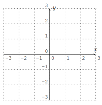
We have seen in the last section that each point on the number line is represented by a real number \(x\) in \(\mathbb{R}\). Similarly, each point in the coordinate plane is represented by a pair of real numbers \((x,y)\). The coordinate plane is denoted by \(\mathbb{R}^{2}\). Here is a picture of the coordinate plane:
In this section, we will discuss the straight line in the coordinate plane. We will discuss its slope and intercepts. We will also discuss the line’s corresponding algebraic forms: the point-slope form and the slope-intercept form.
By drawing a line on a coordinate plane we associate every point on the line with a pair of numbers \((a,b)\), where \(a\) is called the \(x-\)coordinate and \(b\) is called the \(y-\)coordinate. Consider, for example, the picture

We see that \((-2,0)\) lies on the line and so does \((2,2)\). Of course, there are an infinite number of points on the line. This set of points can also be described by an equation relating the \(x-\) and \(y-\) coordinates of points on the line. For example \(2y-x=2\) is the equation of the line above. Notice that \((-2,0)\) satisfies the equation since \(2(0)-(-2)=2\) and \((2,2)\) satisfies the equation since \(2(2)-(2)=2\). It is a fact that every line has an equation of the form \(px+qy=r\), that is, given a line, there are numbers \(p, q\) and \(r\) so that a point \((a,b)\) is on the graph of the line if and only if \(pa+qb=r\).
Notice that, in the example, if we put our finger on \((-2,0)\) and move it up and over to the point \((2,2)\) we have moved \(2\) units up and \(4\) units to the right. If from there (\((2,2)\)) we move another \(2\) units up and \(4\) units to the right then we land again on the line (at \((6,4)\)). In fact no matter where we start on the line if from there we move \(2\) units up and \(4\) units to the right we always land on the line again. The ratio \(\dfrac{\text{rise}}{\text{run}}=\dfrac24\) is called the slope of this line. The word ‘rise’ indicates vertical movement (down being negative) and ‘run’ indicates horizontal movement (left being negative). Notice that \(\dfrac24=\dfrac12=\dfrac{-1}{-2}\) and so on. So we could also see that if we start at \((-2,0)\) and rise \(1\) and run \(2\) we land at \((0,1)\) which is on the line and if we start at \((2,2)\) and rise \(-1\) (move down \(1\)) and run \(-2\) (move to the left \(2\)) we end up at \((0,1)\), which is again on the line.
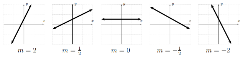
Generally, the slope describes how fast the line grows towards the right. For any two points \(P_1(x_1,y_1)\) and \(P_2(x_2,y_2)\) on the line \(L\), the slope \(m\) is given by the following formula \(\left (\text {which is } \dfrac{\text{rise}}{\text{run}} \right )\):

\[\label{slope} \text{Slope: } \quad\quad \boxed{m=\dfrac{y_2-y_1}{x_2-x_1}}\quad\quad\]
The slope determines how fast a line grows. When the slope \(m\) is negative the line declines towards the right.
From Equation \ref{slope}, we see that for a given slope \(m\) and a point \(P_1(x_1,y_1)\) on the line, any other point \((x,y)\) on the line satisfies \(m=\dfrac{y-y_1}{x-x_1}\). Multiplying \((x-x_1)\) on both sides gives what is called the point-slope form of the line:
\[\label{point-slope-form} \boxed{y-y_1=m\cdot (x-x_1)}\]
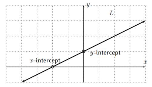
Other prominent features of a graph of a line (or other graphs) include where the graph crosses the \(x\)-axis and the \(y-\)axis. For a given line \(L\), let us recall what the \(x\)- and \(y\)-intercepts are. The \(x\)-intercept is the point on the \(x\)-axis where the line intersects the \(x\)-axis. Similarly, the \(y\)-intercept is the point on the \(y\)-axis where the line intersects the \(y\)-axis.
One way to describe a line using the slope and \(y\)-intercept is the so-called slope-intercept form of the line.
The slope-intercept form of the line is the equation
\[\label{slope-intercept} \boxed{y=m\cdot x+b}\]
Here, \(m\) is the slope and \((0,b)\) is the \(y\)-intercept of the line.
Here is an example of a line in slope-intercept form.
Graph the line \(y=2x+3\).
Solution
We calculate \(y\) for various values of \(x\). For example, when \(x\) is \(-2, -1, 0, 1, 2\), or \(3\), we calculate
\[\begin{array}{|c||c|c|c|c|c|c|}
\hline x & -2 & -1 & 0 & 1 & 2 & 3 \\
\hline \hline y & -1 & 1 & 3 & 5 & 7 & 9 \\
\hline
\end{array} \nonumber \]
In the above table each \(y\) value is calculated by substituting the corresponding \(x\) value into our equation \(y=2x+3\):
\[\begin{array}{llll}
x=-2 & \Longrightarrow & y=2 \cdot(-2)+3=-4+3=-1 \\
x=-1 & \Longrightarrow & y=2 \cdot(-1)+3=-2+3=1 \\
x=0 & \Longrightarrow & y=2 \cdot(0)+3=0+3=3 \\
x=1 & \Longrightarrow & y=2 \cdot(1)+3=2+3=5 \\
x=2 & \Longrightarrow & y=2 \cdot(2)+3=4+3=7 \\
x=3 & \Longrightarrow & y=2 \cdot(3)+3=6+3=9
\end{array} \nonumber \]
In the above calculation, the values for \(x\) were arbitrarily chosen. Since a line is completely determined by knowing two points on it, any two values for \(x\) would have worked for the purpose of graphing the line.
Drawing the above points in the coordinate plane and connecting them gives the graph of the line \(y=2x+3\):
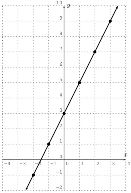
Alternatively, note that the \(y\)-intercept is \((0,3)\) (\(3\) is the additive constant in our initial equation \(y=2x+3\)) and the slope \(m=2\) determines the rate at which the line grows: for each step to the right, we have to move two steps up.
To plot the graph, we first plot the \(y\)-intercept \((0,3)\). Then from that point, rise \(2\) and run \(1\) so that you find yourself at \((1,5)\) (which must be on the graph), and similarly rise \(2\) and run \(1\) to get to \((2,7)\) (which must be on the graph), etc. Plot these points on the graph and connect the dots to form a straight line. As noted above, any \(2\) distinct points on the graph of a straight line are enough to plot the complete line.
Before giving more examples, we briefly want to justify why, in the expression \(y=mx+b\), the number \((0,b)\) is the \(y\)-intercept and \(m\) is the slope. This proof may be skipped on a first reading.
Given the line \(y=mx+b\), we want to calculate its \(y\)-intercept and its slope. The \(y\)-intercept is the value of \(y\) where \(x=0\). Therefore, we have that the \(y-\)coordinate of the \(y\)-intercept is
\[y=m\cdot 0 + b = b \nonumber \]
This shows the first claim.
Next, to see why \(m\) is the slope, note that \(P_1(x_1,y_1)\) lies on the line exactly when \(y_1=m x_1 +b\). Similarly, \(P_2(x_2,y_2)\) lies on the line exactly when \(y_2=m x_2 +b\). Subtracting \(y_1=m x_1 +b\) from \(y_2=m x_2 +b\), we obtain:
\[y_2-y_1= (m x_2+b)-(m x_1+b)=m x_2+ b - m x_1 -b = m\cdot (x_2-x_1).\nonumber \]
Dividing by \((x_2-x_1)\) gives
\[\dfrac{y_2-y_1}{(x_2-x_1)}=\dfrac{m\cdot (x_2-x_1)}{ (x_2-x_1)}=\dfrac m 1 = m \nonumber \]
By Equation \ref{slope} the fraction \(\dfrac{y_2-y_1}{x_2-x_1}\) is the slope, establishing that our \(m\) is indeed the slope, as we claimed.
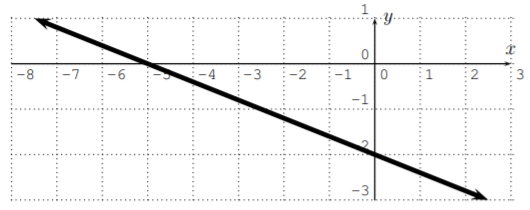
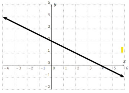
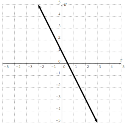
Find the equation of the line in slope-intercept form.
Solution
The \(y\)-intercept can be read off the graph giving us that \(b=2\).
As for the slope, we use formula \ref{slope} and the two points on the line \(P_1(0,2)\) and \(P_2(4,0)\).
We obtain:
\[m=\dfrac{0-2}{4-0}=\dfrac{-2}{4}=-\dfrac{1}{2} \nonumber\]
Thus, the line has the slope-intercept form \(y=-\dfrac 1 2 x +2\).
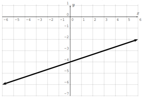
Find the equation of the line in slope-intercept form.
Solution
The \(y\)-intercept is \(b=-4\). To obtain the slope we can again use the \(y\)-intercept \(P_1(0,-4)\). To use \ref{slope}, we need another point \(P_2\) on the line. We may pick any second point on the line, for example, \(P_2(3,-3)\). With this, we obtain
\[m=\dfrac{(-3)-(-4)}{3-0}=\dfrac{-3+4}{3}=\dfrac{1}{3} \nonumber \]
Thus, the line has the slope-intercept form \(y=\dfrac 1 3 x -4\).
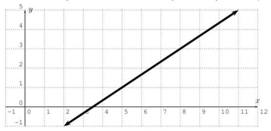
Find the equation of the line in point-slope form \ref{point-slope-form}.
Solution
We need to identify one point \((x_1,y_1)\) on the line together with the slope \(m\) of the line so that we can write the line in point-slope form: \(y-y_1=m(x-x_1)\). By direct inspection, we identify the two points \(P_1(5,1)\) and \(P_2(8,3)\) on the line, and with this we calculate the slope as
\[m=\dfrac{3-1}{8-5}=\dfrac{2}{3} \nonumber \]
Using the point \((5,1)\) we write the line in point-slope form as follows:
\[y-1=\dfrac{2}{3}(x-5) \nonumber \]
Note that our answer depends on the chosen point \((5,1)\) on the line. Indeed, if we choose a different point on the line, such as \((8,3)\), we obtain a different equation, (which nevertheless represents the same line):
\[y-3=\dfrac{2}{3}(x-8) \nonumber \]
Note, that we do not need to solve this for \(y\), since we are looking for an answer in point-slope form.
Find the slope, find the \(y\)-intercept, and graph the line
\[4x+2y -2=0 \nonumber \]
Solution
We first rewrite the equation in slope-intercept form.
\[\begin{aligned}
4 x+2 y-2=0 & \stackrel{(-4 x+2)}{\Longrightarrow} 2 y=-4 x+2 \\
& \stackrel{(\text { divide } 2)}{\Longrightarrow} y=-2 x+1
\end{aligned} \nonumber \]
We see that the slope is \(-2\) and the \(y\)-intercept is \((0,1)\).
We can then plot the \(y-\)intercept \((0,1)\) and use the slope \(m=\dfrac{-2}{1}\) to find another point \((1,-1)\). Plot that point, connect the two plotted points, and extend to see the graph below.
We can also graph by plotting points. We can calculate the \(y\)-values for some \(x\)-values. For example when \(x=-2,-1,\dots,3\), we obtain:
\[\begin{array}{|c||c|c|c|c|c|c|}
\hline x & -2 & -1 & 0 & 1 & 2 & 3 \\
\hline \hline y & 5 & 3 & 1 & -1 & -3 & -5 \\
\hline
\end{array} \nonumber \]
This gives the following graph:
Find the slope, \(y\)-intercept, and graph the line \(5y+2x =-10\).
Solution
Again, we first rewrite the equation in slope-intercept form.
\[\begin{array}{cl}
5 y+2 x=-10 & \stackrel{\text { (subtract } 2 x)}{\Longrightarrow} \quad 5 y=-2 x-10 \\
& \stackrel{(\text { divide } 5)}{\Longrightarrow} \quad y=\dfrac{-2 x-10}{5} \\
& \Longrightarrow \quad y=-\dfrac{2}{5} x-2
\end{array} \nonumber \]
Now, the slope is \(-\dfrac 2 5\) and the \(y\)-intercept is \((0,-2)\).
We can plot the \(y-\)intercept and from there move \(2\) units down and \(5\) units to the right to find another point on the line. The graph is given below.
To graph it by plotting points we need to find points on the line. In fact, any two points will be enough to completely determine the graph of the line. For some “smart” choices of \(x\) or \(y\) the calculation of the corresponding value may be easier than for others. We suggest that you find the \(x-\) and \(y-\)intercepts, i.e., point of the form \((?,0)\) (\(y=0\) in the equation and find \(x\)) and \((0,?)\) (set \(x=0\) in the equation and find \(y\)). Plugging \(x=0\) into \(5y+2x=-10\), we obtain
\[\stackrel{x=0}{\Longrightarrow} 5 y+2 \cdot 0=-10 \quad \Longrightarrow 5 y=-10 \quad \Longrightarrow y=-2 \nonumber \]
Similarly, substituting \(y=0\) into \(5y+2x=-10\) gives
\[\stackrel{y=0}{\Longrightarrow} 5 \cdot 0+2 x=-10 \quad \Longrightarrow 2 x=-10 \quad \Longrightarrow x=-5 \nonumber \]
We obtain the following table:
\[\begin{array}{|c||c|c|}
\hline x & 0 & -5 \\
\hline \hline y & -2 & 0 \\
\hline
\end{array} \nonumber \]
This gives the following graph: