9.3: Optional Section- Graphing Polynomials by Hand

Last updated
Save as PDF

Page ID: 49005

Thomas Tradler and Holly Carley
CUNY New York City College of Technology via New York City College of Technology at CUNY Academic Works

$ \newcommand{\vecs}[1]{\overset { \scriptstyle \rightharpoonup} {\mathbf{#1}} } $ $ \newcommand{\vecd}[1]{\overset{-\!-\!\rightharpoonup}{\vphantom{a}\smash {#1}}} $$\newcommand{\id}{\mathrm{id}}$ $ \newcommand{\Span}{\mathrm{span}}$ $ \newcommand{\kernel}{\mathrm{null}\,}$ $ \newcommand{\range}{\mathrm{range}\,}$ $ \newcommand{\RealPart}{\mathrm{Re}}$ $ \newcommand{\ImaginaryPart}{\mathrm{Im}}$ $ \newcommand{\Argument}{\mathrm{Arg}}$ $ \newcommand{\norm}[1]{\| #1 \|}$ $ \newcommand{\inner}[2]{\langle #1, #2 \rangle}$ $ \newcommand{\Span}{\mathrm{span}}$ $\newcommand{\id}{\mathrm{id}}$ $ \newcommand{\Span}{\mathrm{span}}$ $ \newcommand{\kernel}{\mathrm{null}\,}$ $ \newcommand{\range}{\mathrm{range}\,}$ $ \newcommand{\RealPart}{\mathrm{Re}}$ $ \newcommand{\ImaginaryPart}{\mathrm{Im}}$ $ \newcommand{\Argument}{\mathrm{Arg}}$ $ \newcommand{\norm}[1]{\| #1 \|}$ $ \newcommand{\inner}[2]{\langle #1, #2 \rangle}$ $ \newcommand{\Span}{\mathrm{span}}$$\newcommand{\AA}{\unicode[.8,0]{x212B}}$

In this section we will show how to sketch the graph of a factored polynomial without the use of a calculator.

Example $\PageIndex{1}$

Sketch the graph of the following polynomial without using the calculator: \[p(x)=-2(x+10)^3(x+9)x^2(x-8) \nonumber \]

Solution

Note, that on the calculator it is impossible to get a window which will give all of the features of the graph (while focusing on getting the maximum in view the other features become invisible). We will sketch the graph by hand so that some of the main features are visible. This will only be a sketch and not the actual graph up to scale. Again, the graph can not be drawn to scale while being able to see the features.

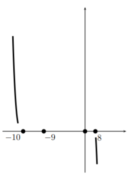
We first start by putting the $x$-intercepts on the graph in the right order, but not to scale necessarily. Then note that

\[p(x)=-2x^7+\dots \text{(lower terms)}\quad \approx -2x^7 \quad\quad \text{ for large }|x| \nonumber \]

This is the leading term of the polynomial (if you expand $p$ it is the term with the largest power) and therefore dominates the polynomial for large $|x|$. So the graph of our polynomial should look something like the graph of $y=-2x^7$ on the extreme left and right side.

$clipboard_ec9d090155983b6200ca81b18373591b0.png$

Now we look at what is going on at the roots. Near each root the factor corresponding to that root dominates. So we have

\[\begin{array}{r|l|l}
\text { for } x \approx & p(x) \approx & \\
\hline-10 & C_{1}(x+10)^{3} & \text { cubic } \\
-9 & C_{2}(x+9) & \text { line } \\
0 & C_{3} x^{2} & \text { parabola } \\
8 & C_{4}(x-8) & \text { line }
\end{array} \nonumber \]

where $C_1, C_2, C_3,$ and $C_4$ are constants which can, but need not, be calculated. For example, whether or not the parabola near $0$ opens up or down will depend on whether the constant $C_3=-2\cdot (0+10)^3(0+9)(0-8)$ is negative or positive. In this case $C_3$ is positive so it opens upward but we will not use this fact to graph. We will see this independently which is a good check on our work.

Starting from the left of our graph where we had determined the behavior for large negative $x$, we move toward the left most zero, $-10$. Near $-10$ the graph looks cubic so we imitate a cubic curve as we pass through $(-10,0)$.

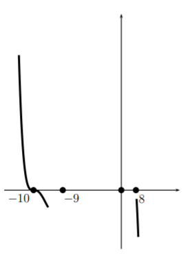
$clipboard_ec2ec7701fee1cc33ae7dfc9cf35a03cc.png$

Now we turn and head toward the next zero, $-9$. Here the graph looks like a line, so we pass through the point $(-9,0)$ as a line would.

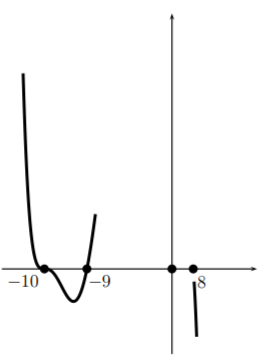
$clipboard_ecb6a6e954ace2a0f14f1a1e4d4f313fc.png$

Now we turn and head toward the root $0$. Here the graph should look like a parabola. So we form a parabola there. (Note that as we had said before the parabola should be opening upward here–and we see that it is).

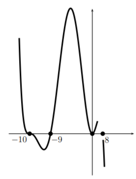
$clipboard_e32117a3e27cf9eeb55d8423ece3ad4b8.png$

Now we turn toward the final zero $8$. We pass through the point $(8,0)$ like a line and we join (perhaps with the use of an eraser) to the large $x$ part of the graph. If this doesn’t join nicely (if the graph is going in the wrong direction) then there has been a mistake. This is a check on your work. Here is the final sketch.

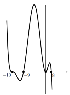
$clipboard_e2222c59a132862518c5e8f758c3b160d.png$

What can be understood from this sketch? Questions like ’when is $p(x)>0$?’ can be answered by looking at the sketch. Further, the general shape of the curve is correct so other properties can be concluded. For example, $p$ has a local minimum between $x=-10$ and $x=-9$ and a local maximum between $x=-9$ and $x=0$, and between $x=0$ and $x=8$. The exact point where the function reaches its maximum or minimum can not be decided by looking at this sketch. But it will help to decide on an appropriate window so that the minimum or maximum finder on the calculator can be used.