9.2: Finding roots of a polynomial with the TI-84
- Page ID
- 49004
\( \newcommand{\vecs}[1]{\overset { \scriptstyle \rightharpoonup} {\mathbf{#1}} } \)
\( \newcommand{\vecd}[1]{\overset{-\!-\!\rightharpoonup}{\vphantom{a}\smash {#1}}} \)
\( \newcommand{\id}{\mathrm{id}}\) \( \newcommand{\Span}{\mathrm{span}}\)
( \newcommand{\kernel}{\mathrm{null}\,}\) \( \newcommand{\range}{\mathrm{range}\,}\)
\( \newcommand{\RealPart}{\mathrm{Re}}\) \( \newcommand{\ImaginaryPart}{\mathrm{Im}}\)
\( \newcommand{\Argument}{\mathrm{Arg}}\) \( \newcommand{\norm}[1]{\| #1 \|}\)
\( \newcommand{\inner}[2]{\langle #1, #2 \rangle}\)
\( \newcommand{\Span}{\mathrm{span}}\)
\( \newcommand{\id}{\mathrm{id}}\)
\( \newcommand{\Span}{\mathrm{span}}\)
\( \newcommand{\kernel}{\mathrm{null}\,}\)
\( \newcommand{\range}{\mathrm{range}\,}\)
\( \newcommand{\RealPart}{\mathrm{Re}}\)
\( \newcommand{\ImaginaryPart}{\mathrm{Im}}\)
\( \newcommand{\Argument}{\mathrm{Arg}}\)
\( \newcommand{\norm}[1]{\| #1 \|}\)
\( \newcommand{\inner}[2]{\langle #1, #2 \rangle}\)
\( \newcommand{\Span}{\mathrm{span}}\) \( \newcommand{\AA}{\unicode[.8,0]{x212B}}\)
\( \newcommand{\vectorA}[1]{\vec{#1}} % arrow\)
\( \newcommand{\vectorAt}[1]{\vec{\text{#1}}} % arrow\)
\( \newcommand{\vectorB}[1]{\overset { \scriptstyle \rightharpoonup} {\mathbf{#1}} } \)
\( \newcommand{\vectorC}[1]{\textbf{#1}} \)
\( \newcommand{\vectorD}[1]{\overrightarrow{#1}} \)
\( \newcommand{\vectorDt}[1]{\overrightarrow{\text{#1}}} \)
\( \newcommand{\vectE}[1]{\overset{-\!-\!\rightharpoonup}{\vphantom{a}\smash{\mathbf {#1}}}} \)
\( \newcommand{\vecs}[1]{\overset { \scriptstyle \rightharpoonup} {\mathbf{#1}} } \)
\( \newcommand{\vecd}[1]{\overset{-\!-\!\rightharpoonup}{\vphantom{a}\smash {#1}}} \)
\(\newcommand{\avec}{\mathbf a}\) \(\newcommand{\bvec}{\mathbf b}\) \(\newcommand{\cvec}{\mathbf c}\) \(\newcommand{\dvec}{\mathbf d}\) \(\newcommand{\dtil}{\widetilde{\mathbf d}}\) \(\newcommand{\evec}{\mathbf e}\) \(\newcommand{\fvec}{\mathbf f}\) \(\newcommand{\nvec}{\mathbf n}\) \(\newcommand{\pvec}{\mathbf p}\) \(\newcommand{\qvec}{\mathbf q}\) \(\newcommand{\svec}{\mathbf s}\) \(\newcommand{\tvec}{\mathbf t}\) \(\newcommand{\uvec}{\mathbf u}\) \(\newcommand{\vvec}{\mathbf v}\) \(\newcommand{\wvec}{\mathbf w}\) \(\newcommand{\xvec}{\mathbf x}\) \(\newcommand{\yvec}{\mathbf y}\) \(\newcommand{\zvec}{\mathbf z}\) \(\newcommand{\rvec}{\mathbf r}\) \(\newcommand{\mvec}{\mathbf m}\) \(\newcommand{\zerovec}{\mathbf 0}\) \(\newcommand{\onevec}{\mathbf 1}\) \(\newcommand{\real}{\mathbb R}\) \(\newcommand{\twovec}[2]{\left[\begin{array}{r}#1 \\ #2 \end{array}\right]}\) \(\newcommand{\ctwovec}[2]{\left[\begin{array}{c}#1 \\ #2 \end{array}\right]}\) \(\newcommand{\threevec}[3]{\left[\begin{array}{r}#1 \\ #2 \\ #3 \end{array}\right]}\) \(\newcommand{\cthreevec}[3]{\left[\begin{array}{c}#1 \\ #2 \\ #3 \end{array}\right]}\) \(\newcommand{\fourvec}[4]{\left[\begin{array}{r}#1 \\ #2 \\ #3 \\ #4 \end{array}\right]}\) \(\newcommand{\cfourvec}[4]{\left[\begin{array}{c}#1 \\ #2 \\ #3 \\ #4 \end{array}\right]}\) \(\newcommand{\fivevec}[5]{\left[\begin{array}{r}#1 \\ #2 \\ #3 \\ #4 \\ #5 \\ \end{array}\right]}\) \(\newcommand{\cfivevec}[5]{\left[\begin{array}{c}#1 \\ #2 \\ #3 \\ #4 \\ #5 \\ \end{array}\right]}\) \(\newcommand{\mattwo}[4]{\left[\begin{array}{rr}#1 \amp #2 \\ #3 \amp #4 \\ \end{array}\right]}\) \(\newcommand{\laspan}[1]{\text{Span}\{#1\}}\) \(\newcommand{\bcal}{\cal B}\) \(\newcommand{\ccal}{\cal C}\) \(\newcommand{\scal}{\cal S}\) \(\newcommand{\wcal}{\cal W}\) \(\newcommand{\ecal}{\cal E}\) \(\newcommand{\coords}[2]{\left\{#1\right\}_{#2}}\) \(\newcommand{\gray}[1]{\color{gray}{#1}}\) \(\newcommand{\lgray}[1]{\color{lightgray}{#1}}\) \(\newcommand{\rank}{\operatorname{rank}}\) \(\newcommand{\row}{\text{Row}}\) \(\newcommand{\col}{\text{Col}}\) \(\renewcommand{\row}{\text{Row}}\) \(\newcommand{\nul}{\text{Nul}}\) \(\newcommand{\var}{\text{Var}}\) \(\newcommand{\corr}{\text{corr}}\) \(\newcommand{\len}[1]{\left|#1\right|}\) \(\newcommand{\bbar}{\overline{\bvec}}\) \(\newcommand{\bhat}{\widehat{\bvec}}\) \(\newcommand{\bperp}{\bvec^\perp}\) \(\newcommand{\xhat}{\widehat{\xvec}}\) \(\newcommand{\vhat}{\widehat{\vvec}}\) \(\newcommand{\uhat}{\widehat{\uvec}}\) \(\newcommand{\what}{\widehat{\wvec}}\) \(\newcommand{\Sighat}{\widehat{\Sigma}}\) \(\newcommand{\lt}{<}\) \(\newcommand{\gt}{>}\) \(\newcommand{\amp}{&}\) \(\definecolor{fillinmathshade}{gray}{0.9}\)We have seen that the roots are important features of a polynomial. Recall that the roots of the polynomial \(f\) are those \(x_0\) for which \(f(x_0)=0\). These are, of course, precisely the \(x\)-intercepts of the graph. Therefore we may use the graph of a polynomial for finding its roots as we did in section 9.1.
Find the roots of the polynomial from its graph.
- \(f(x)=x^3-7x^2+14x-8\)
- \(f(x)=-x^3+8x^2-21x+18\)
- \(f(x)=x^4+3x^3-x+6\)
- \(f(x)=x^5-3x^4-8x^3+24x^2+15x-45\)
Solution
- We start by graphing the polynomial \(f(x)=x^3-7x^2+14x-8\).
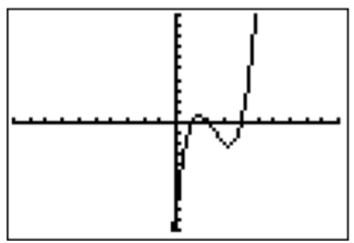
The graph suggests that the roots are at \(x=1\), \(x=2\), and \(x=4\). This may easily be checked by looking at the function table.
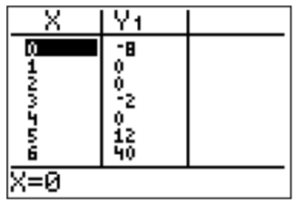
Since the polynomial is of degree \(3\), there cannot be any other roots.
- Graphing \(f(x)=-x^3+8x^2-21x+18\) with the calculator shows the following display.
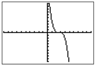
Zooming into the graph reveals that there are in fact two roots, \(x=2\) and \(x=3\), which can be confirmed from the table.

Note, that the root \(x=3\) only “touches” the \(x\)-axis. This is due to the fact that \(x=3\) appears as a multiple root. Indeed, since \(3\) is a root, we can divide \(f(x)\) by \(x-3\) without remainder and factor the resulting quotient to see that that
\[f(x)=(x-2)(x-3)(x-3)=(x-2)(x-3)^2 \nonumber \]
We say that \(x=3\) is a root of multiplicity \(2\).
- The graph of \(f(x)=x^4+3x^3-x+6\) in the standard window is displayed as follows.
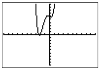
Since this is a polynomial of degree \(4\), all of the essential features are already displayed in the above graph. The roots can be seen by zooming into the graph.

From the table and the graph we see that there is a root at \(x=-2\) and another root at between \(-3\) and \(-2\). Finding the exact value of this second root can be quite difficult, and we will say more about this in section 2 below. At this point, we can only approximate the root with the “zero” function from the “calc” menu:

- The graph of \(f(x)=x^5-3x^4-8x^3+24x^2+15x-45\) in the standard window is displayed below.
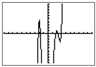
Zooming into the \(x\)-axis, and checking the table shows that the only obvious root is \(x=3\).

The other four roots are more difficult to find. However they can be approximated using the “zero” function from the “calc” menu.
It will often be necessary to find the roots of a quadratic polynomial. For this reason, we recall the well-known quadratic formula.
The solutions of the equation \(f(x)=ax^2+bx+c\) for some real numbers \(a\), \(b\), and \(c\) are given by:
\[x_{1}=\dfrac{-b+\sqrt{b^{2}-4 a c}}{2 a}, \quad \text { and } \quad x_{2}=\dfrac{-b-\sqrt{b^{2}-4 a c}}{2 a} \nonumber \]
We may combine the two solutions \(x_1\) and \(x_2\) and simply write this as:
\[\boxed{x_{1 / 2}=\dfrac{-b \pm \sqrt{b^{2}-4 a c}}{2 a}} \nonumber \]
We may always use the roots \(x_1\) and \(x_2\) of a quadratic polynomial \(f(x)=ax^2+bx+c\) from the quadratic formula and rewrite the polynomial as:
\[\boxed{f(x)=a x^{2}+b x+c=a \cdot\left(x-\frac{-b+\sqrt{b^{2}-4 a c}}{2 a}\right)\left(x-\frac{-b-\sqrt{b^{2}-4 a c}}{2 a}\right)} \nonumber \]


