9.1: Graphs of polynomials

We now discuss the shape of the graphs of polynomial functions. Recall that a polynomial function $f$ of degree $n$ is a function of the form

$$f(x)=a_n x^n+a_{n-1} x^{n-1}+\dots +a_2 x^2+ a_1 x + a_0 \nonumber$$

Observation: Graphs of Polynomials

We already know from Section 2.1, that the graphs of polynomials $f(x)=ax+b$ of degree $1$ are straight lines.

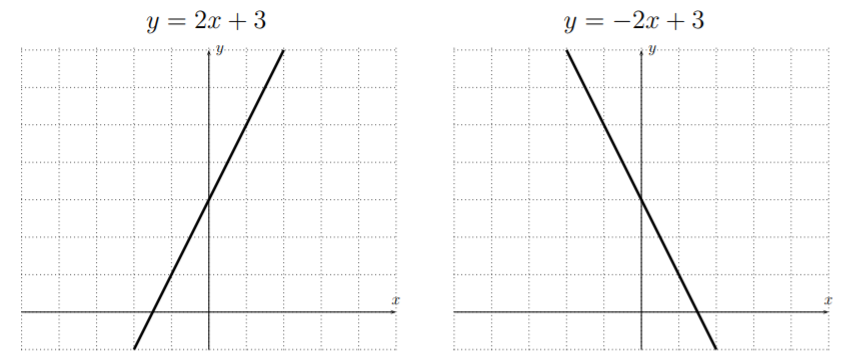
Polynomials of degree $1$ have only one root.

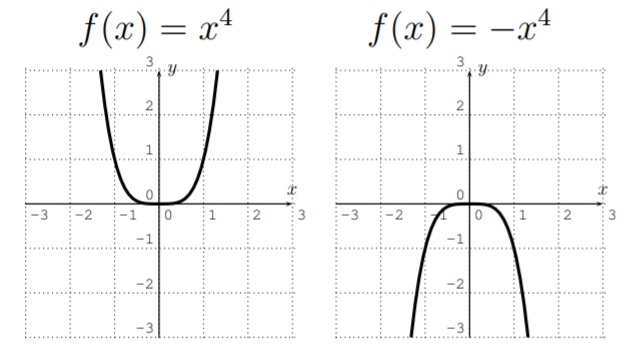
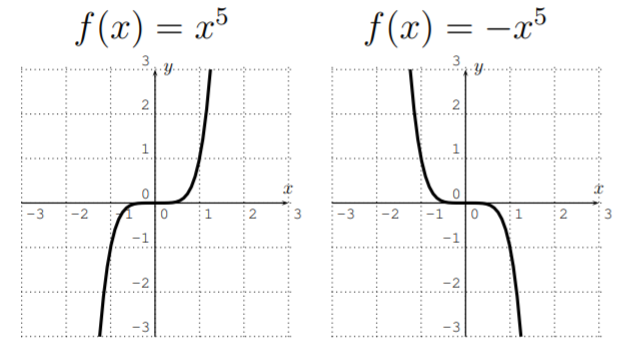
It is also easy to sketch the graphs of functions $f(x)=x^n$.

Observation: Graph of Function $f(x)=x^n$

Graphing $y=x^2$, $y=x^3$, $y=x^4$, $y=x^5$, we obtain:

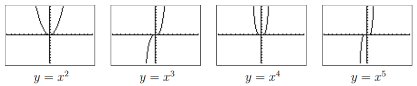
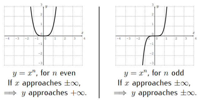
From this, we see that the shape of the graph of $f(x)=x^n$ depends on $n$ being even or odd.

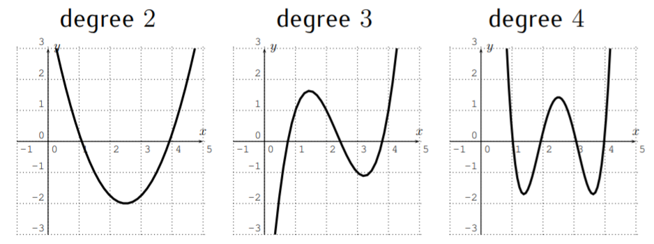
We now make some observations about graphs of general polynomials of degrees $2$, $3$, $4$, $5$, and, more generally, of any degree $n$. In particular, we will be interested in the number of roots and the number of extrema (that is the number of maxima or a minima) of the graph of a polynomial $f$.

Observation: Graph of Parabola

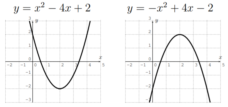
Let $f(x)=ax^2+bx+c$ be a polynomial of degree $2$. The graph of $f$ is a parabola.

• $f$ has at most $2$ roots. $f$ has one extremum (that is one maximum or minimum).

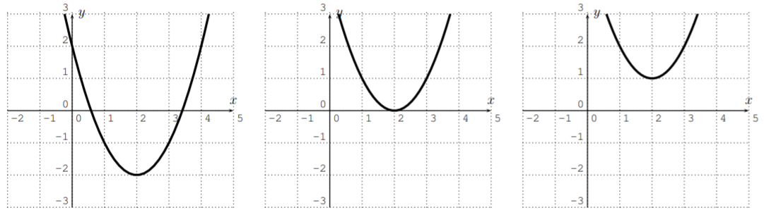
• If $a>0$ then $f$ opens upwards, if $a<0$ then $f$ opens downwards.

Observation: Graph of Polynomial of degree $3$

Let $f(x)=ax^3+bx^2+cx+d$ be a polynomial of degree $3$. The graph may change its direction at most twice.

• $f$ has at most $3$ roots. $f$ has at most $2$ extrema.

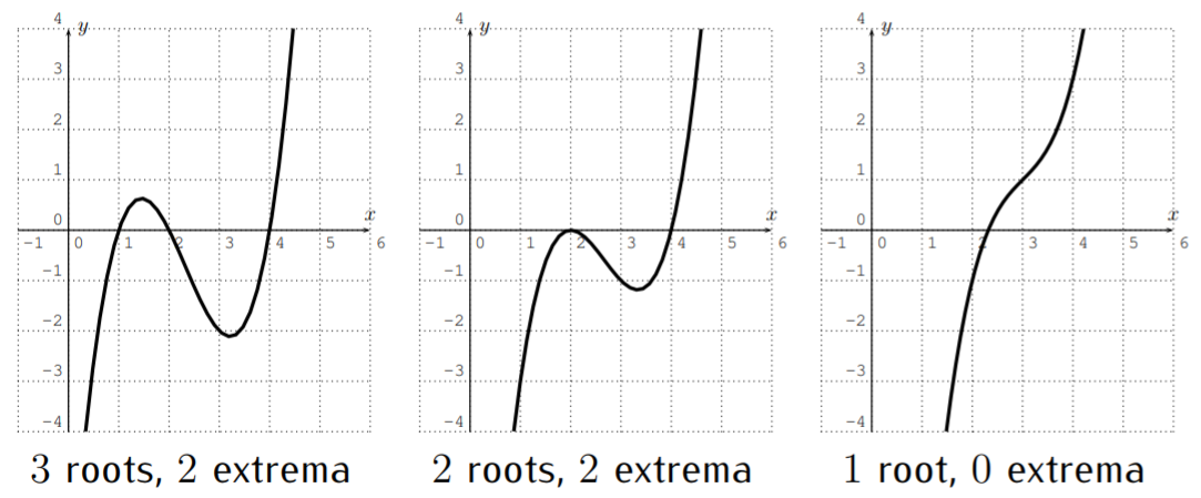
• If $a>0$ then $f(x)$ approaches $+\infty$ when $x$ approaches $+\infty$ (that is, $f(x)$ gets large when $x$ gets large), and $f(x)$ approaches $-\infty$ when $x$ approaches $-\infty$. If $a<0$ then $f(x)$ approaches $-\infty$ when $x$ approaches $+\infty$, and $f(x)$ approaches $+\infty$ when $x$ approaches $-\infty$.

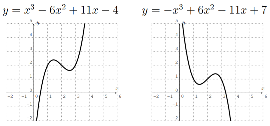
Above, we have a first instance of a polynomial of degree $n$ which “changes its direction” one more time than a polynomial of one lesser degree $n-1$. Below, we give examples of this phenomenon for higher degrees as well.

Observation: Graph of Polynomial of degree $4$

Let $f(x)=ax^4+bx^3+cx^2+dx+e$ be a polynomial of degree $4$.

• $f$ has at most $4$ roots. $f$ has at most $3$ extrema. If $a>0$ then $f$ opens upwards, if $a<0$ then $f$ opens downwards.

Observation: Graph of Polynomial of degree $5$

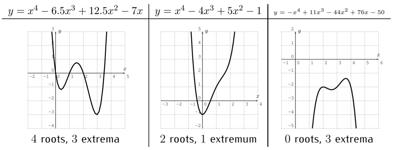
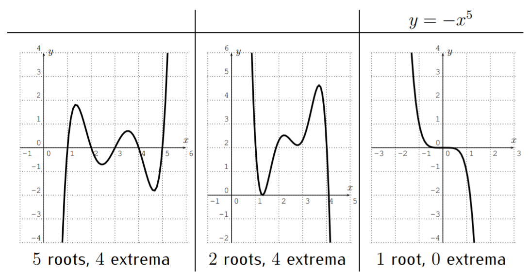
Let $f$ be a polynomial of degree $5$.

• $f$ has at most $5$ roots. $f$ has at most $4$ extrema. If $a>0$ then $f(x)$ approaches $+\infty$ when $x$ approaches $+\infty$, and $f(x)$ approaches $-\infty$ when $x$ approaches $-\infty$. If $a<0$ then $f(x)$ approaches $-\infty$ when $x$ approaches $+\infty$, and $f(x)$ approaches $+\infty$ when $x$ approaches $-\infty$.

Observation: Graph of Polynomial of degree $n$

• Let $f(x)=a_n x^n+a_{n-1} x^{n-1}+\dots +a_2 x^2+ a_1 x + a_0$ be a polynomial of degree $n$. Then $f$ has at most $n$ roots, and at most $n-1$ extrema.

• Assume the degree of $f$ is even $n=2, 4, 6, \dots$. If $a_n>0$, then the polynomial opens upwards. If $a_n<0$ then the polynomial opens downwards.

• Assume the degree of $f$ is odd, $n=1, 3, 5, \dots$. If $a_n>0$, then $f(x)$ approaches $+\infty$ when $x$ approaches $+\infty$, and $f(x)$ approaches $-\infty$ as $x$ approaches $-\infty$. If $a_n<0$, then $f(x)$ approaches $-\infty$ when $x$ approaches $+\infty$, and $f(x)$ approaches $+\infty$ as $x$ approaches $-\infty$.

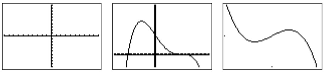
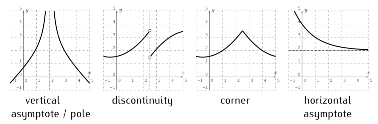
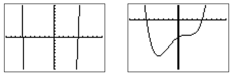
• The domain of a polynomial $f$ is all real numbers, and $f$ is continuous for all real numbers (there are no jumps in the graph). The graph of $f$ has no horizontal or vertical asymptotes, no discontinuities (jumps in the graph), and no corners. Furthermore, $f(x)$ approaches $\pm \infty$ when $x$ approaches $\pm \infty$. Therefore, the following graphs cannot be graphs of polynomials.

Example $\PageIndex{1}$

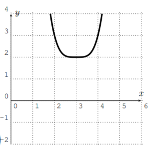
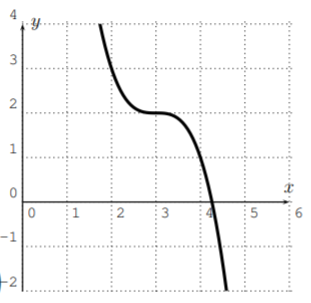
Which of the following graphs could be the graphs of a polynomial? If the graph could indeed be a graph of a polynomial then determine a possible degree of the polynomial.

1. 
2. 
3. 
4. 
5. 

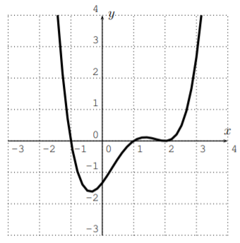
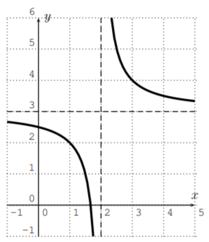
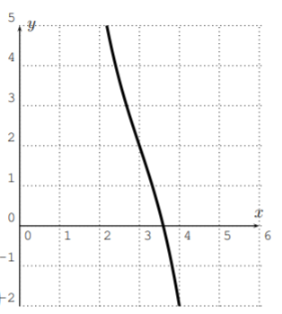
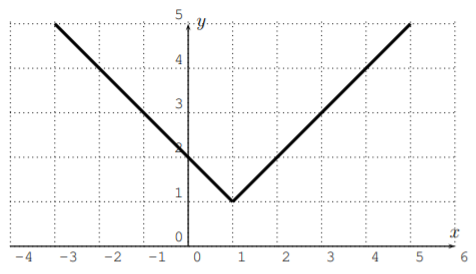
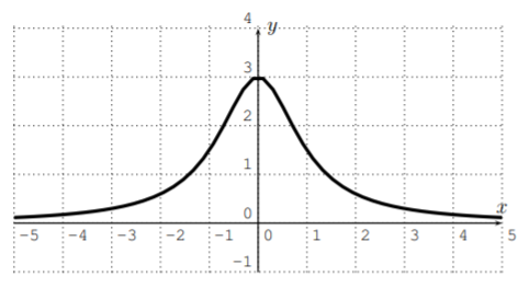
Solution

1. Yes, this could be a polynomial. The degree could be, for example, $4$.
2. No, since the graph has a pole.
3. Yes, this could be a polynomial. A possible degree would be degree $3$.
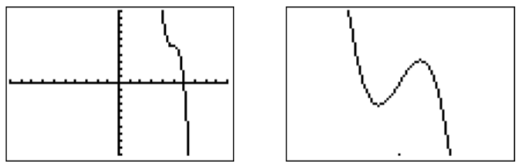
4. No, since the graph has a corner.
5. No, since $f(x)$ does not approach $\infty$ or $-\infty$ as $x$ approaches $\infty$. (In fact $f(x)$ approaches $0$ as $x$ approaches $\pm\infty$ and we say that the function (or graph) has a horizontal asymptote $y=0$.)

Example $\PageIndex{2}$

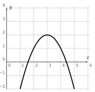
Identify the graphs of the polynomials in (a), (b) and (c) with the functions (i), (ii), and (iii).

1. 
2. 
3. 

1. $f(x)=-x^3+9x^2-27x+29$
2. $f(x)=-x^2+6x-7$
3. $f(x)=x^4-12x^3+54x^2-108x+83$

Solution

The only odd degree function is (i) and it must therefore correspond to graph (c). For (ii), since the leading coefficient is negative, we know that the function opens downwards, so that it corresponds to graph (a). Finally (iii) opens upwards, since the leading coefficient is positive, so that its graph is (b).

When graphing a function, we need to make sure to draw the function in a window that expresses all the interesting features of the graph. More precisely, we need to make sure that the graph includes all essential parts of the graph, such as all intercepts (both $x$-intercepts and $y$-intercept), all roots, all asymptotes (this will be discussed in the next part), and the long range behavior of the function (that is how the function behaves when $x$ approaches $\pm \infty$). We also want to include all extrema (that is all maxima and minima) of the function.

Example $\PageIndex{3}$

Graph of the given function with the TI-84. Include all extrema and intercepts of the graph in your viewing window.

1. $f(x)=-x^3+26x^2-129x+175$
2. $f(x)=.1x^4-2.4x^2+6.4x-35$
3. $f(x)=-5x^3+75x^2-374.998x+630$
4. $f(x)=-.01x^4+.4x^3+.0025x^2-160x+1600$

Solution

1. The graph in the standard window looks as follows:

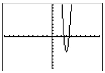
However, since the function is of degree $3$, this cannot be the full graph, as $f(x)$ has to approach $-\infty$ when $x$ approaches $\infty$. Zooming out, and rescaling appropriately for the following setting the following graph.

2. The graph in the standard window is drawn on the left below. After rescaling to $-10\leq x\leq 10$ and $-100 \leq y\leq 30$ we obtain the graph on the right.

3. The graph in the standard window is drawn on the left. Zooming to the interesting part of the graph, we obtain the graph on the right. (Below, we have chosen a window of $4.94\leq x\leq 5.06$ and $5.00995 \leq y\leq 5.01005$.)

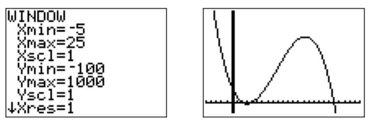
4. The standard window (see left graph) shows an empty coordinate system without any part of the graph. However, zooming out to $-30\leq x\leq 40$ and $-1000 \leq y\leq 4000$, we obtain the middle graph. There is another interesting part of the graph displayed on the right, coming from zooming to the plateau on the right (here shown at $19.2\leq x\leq 20.8$ and $0.9 \leq y\leq 1.1$).