22.2: Operations on vectors

There are two basic operations on vectors, which are the scalar multiplication and the vector addition. We start with the scalar multiplication.

Definition: Scalar Multiplication

The scalar multiplication of a real number \(r\) with a vector \(\vec{v}=\langle a,b\rangle\) is defined to be the vector given by multiplying \(r\) to each coordinate.

\[\boxed{ r\cdot \langle a,b \rangle := \langle r\cdot a, r \cdot b \rangle }\]

We study the effect of scalar multiplication with an example.

Example \(\PageIndex{1}\)

Multiply, and graph the vectors.

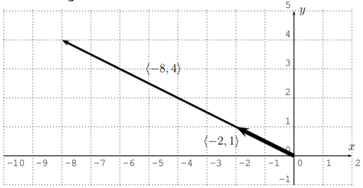
1. \(4\cdot \langle-2,1\rangle\)
2. \((-3)\cdot \langle -6,-2 \rangle\)

Solution

1. The calculation is straightforward.

\[4\cdot \langle-2,1\rangle=\langle4\cdot (-2),4\cdot 1\rangle=\langle-8,4\rangle \nonumber \]

The vectors are displayed below. We see, that \(\langle-2,1\rangle\) and \(\langle-8,4\rangle\) both have the same directional angle, and the latter stretches the former by a factor \(4\).

2. Algebraically, we calculate the scalar multiplication as follows:

\[(-3)\cdot \langle -6,-2 \rangle= \langle (-3)\cdot(-6),(-3)\cdot(-2) \rangle =\langle 18,6 \rangle \nonumber \]

Furthermore, graphing the vectors gives:

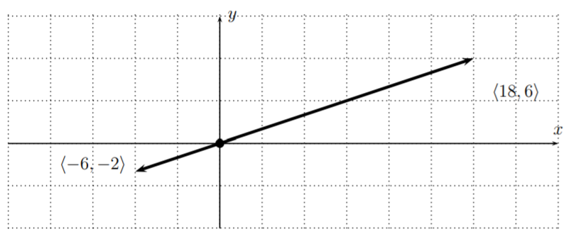
We see that the directional angle of the two vectors differs by \(180^\circ\). Indeed, \(\langle18,6\rangle\) is obtained from \(\langle -6,-2\rangle\) by reflecting it at the origin \(O(0,0)\) and then stretching the result by a factor \(3\).

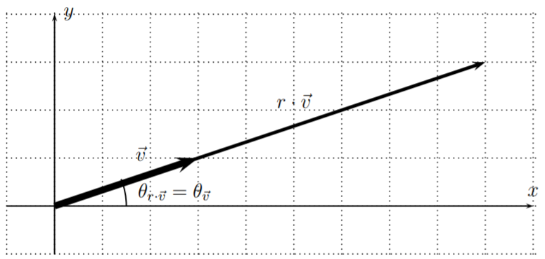
We see from the above example, that scalar multiplication by a positive number \(c\) does not change the angle of the vector, but it multiplies the magnitude by \(c\).

Observation: c-times-vector

Let \(\vec{v}\) be a vector with magnitude \(||\vec{v}||\) and angle \(\theta_{\vec{v}}\). Then, for a positive scalar, \(r>0\), the scalar multiple \(r\cdot \vec{v}\) has the same angle as \(\vec{v}\), and a magnitude that is \(r\) times the magnitude of \(\vec{v}\):

\[\text{for $r>0$: } \quad ||r\cdot \vec{v}|| = r\cdot ||\vec{v}|| \quad\text{ and } \quad \theta_{r\cdot \vec{v}}=\theta_{\vec{v}}\]

Definition: Unit Vector

A vector \(\vec{u}\) is called a unit vector, if it has a magnitude of \(1\).

\[\vec{u} \text{ is a unit vector } \quad \iff \quad ||\vec{u}||=1\]

There are two special unit vectors, which are the vectors pointing in the \(x\)- and the \(y\)-direction.

\[\boxed{\vec{i}:=\langle 1,0\rangle}\quad \text{ and }\quad \boxed{\vec{j}:=\langle 0,1\rangle}\]

Example \(\PageIndex{2}\)

Find a unit vector in the direction of \(\vec{v}\).

1. \(\langle 8, 6 \rangle\)
2. \(\langle -2,3\sqrt{7} \rangle\)

Solution

1. Note that the magnitude of \(\vec{v}=\langle 8, 6 \rangle\) is

\[||\langle 8, 6 \rangle||=\sqrt{8^2+6^2}=\sqrt{64+36}=\sqrt{100}=10 \nonumber \]

Therefore, if we multiply \(\langle 8, 6 \rangle\) by \(\dfrac{1}{10}\) we obtain \(\dfrac{1}{10}\cdot \langle 8, 6 \rangle=\langle \dfrac{8}{10}, \dfrac{6}{10} \rangle=\langle \dfrac{4}{5}, \dfrac{3}{5} \rangle\), which (according to Observation [OBS:c-times-vector] above) has the same directional angle as \(\langle 8, 6 \rangle\), and has a magnitude of \(1\):

\[\left|\left|\dfrac{1}{10}\cdot \langle 8, 6 \rangle\right|\right| = \dfrac{1}{10}\cdot ||\langle 8, 6 \rangle||=\dfrac{1}{10}\cdot 10=1 \nonumber \]

2. The magnitude of \(\langle -2,3\sqrt{7} \rangle\) is

\[||\langle -2,3\sqrt{7} \rangle||=\sqrt{(-2)^2+(3\sqrt{7})^2}=\sqrt{4+9\cdot 7}=\sqrt{4+63}=\sqrt{67} \nonumber\]

Therefore, we have the unit vector

\[\dfrac{1}{\sqrt{67}}\cdot \langle -2,3\sqrt{7} \rangle=\langle \dfrac{-2}{\sqrt{67}},\frac{3\sqrt{7} }{\sqrt{67}}\rangle=\langle \dfrac{-2\sqrt{67}}{67},\dfrac{3\sqrt{7}\sqrt{67}}{67}\rangle=\langle \dfrac{-2\sqrt{67}}{67},\dfrac{3\sqrt{469}}{67}\rangle \nonumber\]

which again has the same directional angle as \(\langle -2,3\sqrt{7} \rangle\). Now, \(\dfrac{1}{\sqrt{67}}\cdot \langle -2,3\sqrt{7} \rangle\) is a unit vector, since \[||\dfrac{1}{\sqrt{67}}\cdot \langle -2,3\sqrt{7} \rangle||=\dfrac{1}{\sqrt{67}}\cdot ||\langle -2,3\sqrt{7} \rangle||=\dfrac{1}{\sqrt{67}}\cdot \sqrt{67}=1 \nonumber \]

The second operation on vectors is vector addition, which we discuss now.

Definition: Vector Addition

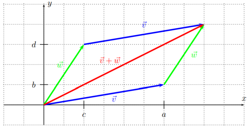
Let \(\vec{v}=\langle a,b \rangle\) and \(\vec{w}=\langle c,d \rangle\) be two vectors. Then the vector addition \(\vec{v}+\vec{w}\) is defined by component-wise addition:

\[\boxed{\,\, \langle a,b \rangle+\langle c,d \rangle:=\langle a+c,b+d \rangle \,\,}\]

In terms of the plane, the vector addition corresponds to placing the vectors \(\vec{v}\) and \(\vec{w}\) as the edges of a parallelogram, so that \(\vec{v}+\vec{w}\) becomes its diagonal. This is displayed below.

Example \(\PageIndex{3}\)

Perform the vector addition and simplify as much as possible.

1. \(\langle 3,-5 \rangle+\langle 6,4 \rangle\)
2. \(5\cdot \langle -6,2 \rangle-7\cdot \langle 1, -3 \rangle\)
3. \(4\vec{i}+9\vec{j}\)
4. Find \(2\vec{v}+3\vec{w}\) for \(\vec{v}=-6\vec{i}-4\vec{j}\) and \(\vec{w}=10\vec{i}-7\vec{j}\)
5. Find \(-3\vec{v}+5\vec{w}\) for \(\vec{v}=\langle 8,\sqrt{3} \rangle\) and \(\vec{w}=\langle 0,4\sqrt{3} \rangle\)

Solution

We can find the answer by direct algebraic computation.

1. \(\langle 3,-5\rangle+\langle 6,4\rangle=\langle 3+6,-5+4\rangle=\langle 9,-1\rangle\)
2. \(5 \cdot\langle-6,2\rangle-7 \cdot\langle 1,-3\rangle=\langle-30,10\rangle+\langle-7,21\rangle=\langle-37,31\rangle\)
3. \(4 \vec{i}+9 \vec{j}=4 \cdot\langle 1,0\rangle+9 \cdot\langle 0,1\rangle=\langle 4,0\rangle+\langle 0,9\rangle=\langle 4,9\rangle\)

From the last calculation, we see that every vector can be written as a linear combination of the vectors \(\vec{i}\) and \(\vec{j}\).

\[\boxed{\langle a,b \rangle = a\cdot \vec{i}+b\cdot \vec{j}} \nonumber\]

We will use this equation for the next example (d). Here, \(\vec{v}=-6\vec{i}-4\vec{j}=\langle-6,-4\rangle\) and \(\vec{w}=10\vec{i}-7\vec{j}=\langle 10,-7\rangle\). Therefore, we obtain:

4. \(2 \vec{v}+3 \vec{w}=2 \cdot\langle-6,-4\rangle+3 \cdot\langle 10,-7\rangle=\langle-12,-8\rangle+\langle 30,-21\rangle=\langle 18,-29\rangle\)

5. \(\begin{aligned}-3 \vec{v}+5 \vec{w} &=-3 \cdot\langle 8, \sqrt{3}\rangle+5 \cdot\langle 0,4 \sqrt{3}\rangle\\&=\langle-24,-3 \sqrt{3}\rangle+\langle 0,20 \sqrt{3}\rangle \\&=\langle-24,17 \sqrt{3}\rangle\end{aligned}\)

Note that the answer could also be written as \(-3\vec{v}+5\vec{w}=-24\vec{i}+17\sqrt{3}\vec{j}\).

In many applications in the sciences, vectors play an important role, since many quantities are naturally described by vectors. Examples for this in physics include the velocity \(\vec{v}\), acceleration \(\vec{a}\), and the force \(\vec{F}\) applied to an object. [EXA:addition-of-forces] The forces \(\vec{F_1}\) and \(\vec{F_2}\) are applied to an object.

Example \(\PageIndex{4}\)

Find the resulting total force \(\vec{F}=\vec{F_1}+\vec{F_2}\). Determine the magnitude and directional angle of the total force \(\vec{F}\). Approximate these values as necessary. Recall that the international system of units for force is the newton \([1N=1\frac{kg\cdot m}{s^2}]\).

1. \(\vec{F_1}\) has magnitude \(3\) newtons, and angle \(\theta_1=45^\circ\), \(\vec{F_2}\) has magnitude \(5\) newtons, and angle \(\theta_2=135^\circ\)
2. \(||\vec{F_1}||=7\) newtons, and \(\theta_1=\dfrac{\pi}{6}\), and \(||\vec{F_2}||=4\) newtons, and \(\theta_2=\dfrac{5\pi}{3}\)

Solution

1. The vectors \(\vec{F_1}\) and \(\vec{F_2}\) are given by their magnitudes and directional angles. However, the addition of vectors (in Definition [DEF:vector-addition]) is defined in terms of their components. Therefore, our first task is to find the vectors in component form. As was stated in equation 22.1.2 [EQU:magnitude-angle-to-component] on page , the vectors are calculated by \(\vec{v}=\langle \,\,\, ||\vec{v}||\cdot \cos(\theta)\,\,\, , \,\,\, ||\vec{v}||\cdot \sin(\theta) \,\,\, \rangle\). Therefore,

\[\begin{aligned} \vec{F_1} &= \langle 3\cdot \cos(45^\circ), 3\cdot \sin(45^\circ) \rangle= \langle 3\cdot \dfrac{\sqrt{2}}{2}, 3\cdot \dfrac{\sqrt{2}}{2} \rangle= \langle \dfrac{3\sqrt{2}}{2}, \dfrac{3\sqrt{2}}{2} \rangle \\ \vec{F_2} &= \langle 5\cdot \cos(135^\circ), 5\cdot \sin(135^\circ) \rangle= \langle 5\cdot \dfrac{-\sqrt{2}}{2}, 5\cdot \dfrac{\sqrt{2}}{2} \rangle =\langle \dfrac{-5\sqrt{2}}{2}, \dfrac{5\sqrt{2}}{2} \rangle\end{aligned} \nonumber \]

The total force is the sum of the forces.

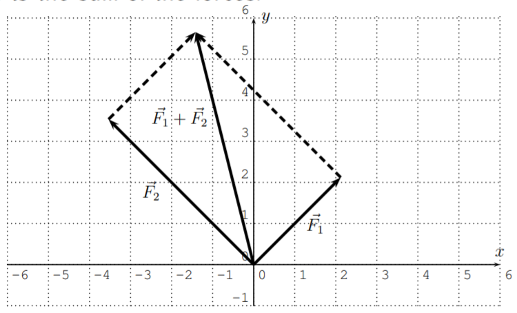
\[\begin{aligned} \vec{F}&=\vec{F_1}+\vec{F_2}\\& = \langle \dfrac{3\sqrt{2}}{2}, \dfrac{3\sqrt{2}}{2} \rangle+\langle \dfrac{-5\sqrt{2}}{2}, \dfrac{5\sqrt{2}}{2} \rangle \\ &= \langle \dfrac{3\sqrt{2}}{2}+\dfrac{-5\sqrt{2}}{2}, \dfrac{3\sqrt{2}}{2} +\dfrac{5\sqrt{2}}{2}\rangle\\& =\langle \dfrac{3\sqrt{2}-5\sqrt{2}}{2}, \dfrac{3\sqrt{2}+5\sqrt{2}}{2}\rangle \\ &= \langle \dfrac{-2\sqrt{2}}{2}, \dfrac{8\sqrt{2}}{2}\rangle\\& = \langle -\sqrt{2}, 4\sqrt{2}\rangle \end{aligned} \nonumber \]

The total force applied in components is \(\vec{F}=\langle -\sqrt{2}, 4\sqrt{2}\rangle\). It has a magnitude of \(||\vec{F}||=\sqrt{(-\sqrt{2})^2+(4\sqrt{2})^2}=\sqrt{2+16\cdot 2}=\sqrt{34}\approx 5.83\) newton. The directional angle is given by \(\tan(\theta)=\dfrac{4\sqrt{2}}{-\sqrt{2}}=-4\). Since \(\tan^{-1}(-4)\approx -76.0^\circ\) is in quadrant IV, and \(\vec{F}=\langle -\sqrt{2}, 4\sqrt{2} \rangle\) is in quadrant II, we see that the directional angle of \(\vec{F}\) is

\[\theta=180^\circ+\tan^{-1}(-4)\approx180^\circ-76.0^\circ \approx 104^\circ \nonumber \]

2. We solve this example in much the same way we solved part (a). First, \(\vec{F_1}\) and \(\vec{F_2}\) in components is given by

\[\begin{aligned} \vec{F_1} &= \langle 7\cdot \cos\Big(\dfrac{\pi}{6}\Big), 7\cdot \sin\Big(\dfrac{\pi}{6}\Big) \rangle= \langle 7\cdot \dfrac{\sqrt{3}}{2}, 7\cdot \dfrac{1}{2} \rangle= \langle \dfrac{7\sqrt{3}}{2}, \dfrac{7}{2} \rangle \\ \vec{F_2} &=\langle 4\cdot \cos\Big(\dfrac{5\pi}{3}\Big), 4\cdot \sin\Big(\dfrac{5\pi}{3}\Big) \rangle= \langle 4\cdot \dfrac{1}{2}, 4\cdot \dfrac{-\sqrt{3}}{2} \rangle= \langle 2, -2\sqrt{3} \rangle\end{aligned} \nonumber \]

The total force is therefore:

\[\begin{aligned} \vec{F}&= \vec{F_1}+\vec{F_2}\\&=\langle \dfrac{7\sqrt{3}}{2}, \dfrac{7}{2} \rangle +\langle 2, -2\sqrt{3} \rangle\\&=\langle \dfrac{7\sqrt{3}}{2}+2, \dfrac{7}{2}-2\sqrt{3} \rangle \\ &\approx \langle 8.06, 0.04 \rangle\end{aligned} \nonumber \]

The magnitude is approximately

\[||\vec{F}||\approx \sqrt{(8.06)^2+(0.04)^2}\approx 8.06 \text{ newton} \nonumber \]

The directional angle is given by \(\tan(\theta)\approx \dfrac{0.04}{8.06}\). Since \(\vec{F}\) is in quadrant I, we see that \(\theta\approx \tan^{-1}\left(\dfrac{0.04}{8.06}\right)\approx 0.3^\circ\).

Note

There is an abstract notion of a vector space. Although we do not use this structure for any further computations, we will state its definition. A vector space is a set \(V\), with the following structures and properties. The elements of \(V\) are called vectors, denoted by the usual symbol \(\vec{v}\). For any vectors \(\vec{v}\) and \(\vec{w}\) there is a vector \(\vec{v}+\vec{w}\), called the vector addition. For any real number \(r\) and vector \(\vec{v}\), there is a vector \(r\cdot \vec{v}\) called the scalar product. These operations have to satisfy the following properties.

Associativity: \((\vec{u}+\vec{v})+\vec{w}=\vec{u}+(\vec{v}+\vec{w})\)

Commutativity: \(\vec{v}+\vec{w}=\vec{w}+\vec{v}\)

Zero element: there is a vector \(\vec{o}\) such that \(\vec{o}+\vec{v}=\vec{v}\) and \(\vec{v}+\vec{o}=\vec{v}\) for every vector \(\vec{v}\)

Negative element: for every \(\vec{v}\) there is a vector \(-\vec{v}\) such that \(\vec{v}+(-\vec{v})=\vec{o}\) and \((-\vec{v})+\vec{v}=\vec{o}\)

Distributivity (1): \(r\cdot (\vec{v}+\vec{w})=r\cdot \vec{v}+ r\cdot \vec{w}\)

Distributivity (2): \((r+ s)\cdot \vec{v}=r\cdot \vec{v}+ s\cdot \vec{v}\)

Scalar compatibility: \((r\cdot s)\cdot \vec{v}=r\cdot (s\cdot \vec{v})\)

Identity: \(1\cdot \vec{v}=\vec{v}\)

A very important example of a vector space is the \(2\)-dimensional plane \(V=\mathbb{R}^2\) as it was discussed in this chapter.