8.6: Parametric Equations

Learning Objectives

• Parameterize a curve.
• Eliminate the parameter.
• Find a rectangular equation for a curve defined parametrically.
• Find parametric equations for curves defined by rectangular equations.

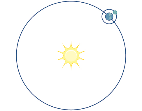
Consider the path a moon follows as it orbits a planet, which simultaneously rotates around the sun, as seen in Figure \(\PageIndex{1}\). At any moment, the moon is located at a particular spot relative to the planet. But how do we write and solve the equation for the position of the moon when the distance from the planet, the speed of the moon’s orbit around the planet, and the speed of rotation around the sun are all unknowns? We can solve only for one variable at a time.

Figure \(\PageIndex{1}\)

In this section, we will consider sets of equations given by \(x(t)\) and \(y(t)\) where \(t\) is the independent variable of time. We can use these parametric equations in a number of applications when we are looking for not only a particular position but also the direction of the movement. As we trace out successive values of \(t\), the orientation of the curve becomes clear. This is one of the primary advantages of using parametric equations: we are able to trace the movement of an object along a path according to time. We begin this section with a look at the basic components of parametric equations and what it means to parameterize a curve. Then we will learn how to eliminate the parameter, translate the equations of a curve defined parametrically into rectangular equations, and find the parametric equations for curves defined by rectangular equations.

Parameterizing a Curve

When an object moves along a curve—or curvilinear path—in a given direction and in a given amount of time, the position of the object in the plane is given by the \(x\)-coordinate and the \(y\)-coordinate. However, both \(x\) and \(y\) vary over time and so are functions of time. For this reason, we add another variable, the parameter, upon which both \(x\) and \(y\) are dependent functions. In the example in the section opener, the parameter is time, \(t\). The \(x\) position of the moon at time, \(t\), is represented as the function \(x(t)\), and the \(y\) position of the moon at time, \(t\), is represented as the function \(y(t)\). Together, \(x(t)\) and \(y(t)\) are called parametric equations, and generate an ordered pair \((x(t), y(t))\). Parametric equations primarily describe motion and direction.

When we parameterize a curve, we are translating a single equation in two variables, such as \(x\) and \(y\),into an equivalent pair of equations in three variables, \(x\), \(y\), and \(t\). One of the reasons we parameterize a curve is because the parametric equations yield more information: specifically, the direction of the object’s motion over time.

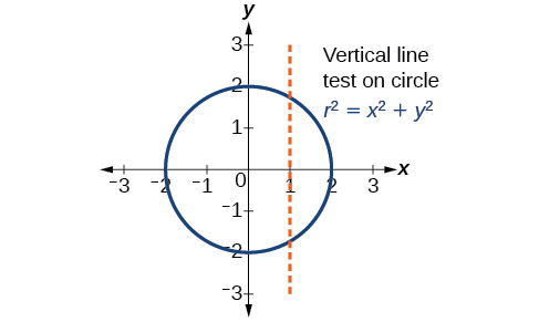
When we graph parametric equations, we can observe the individual behaviors of \(x\) and of \(y\). There are a number of shapes that cannot be represented in the form \(y=f(x)\), meaning that they are not functions. For example, consider the graph of a circle, given as \(r^2=x^2+y^2\). Solving for \(y\) gives \(y=\pm \sqrt{r^2−x^2}\), or two equations: \(y_1=\sqrt{r^2−x^2}\) and \(y_2=−\sqrt{r^2−x^2}\). If we graph \(y_1\) and \(y_2\) together, the graph will not pass the vertical line test, as shown in Figure \(\PageIndex{2}\). Thus, the equation for the graph of a circle is not a function.

Figure \(\PageIndex{2}\)

However, if we were to graph each equation on its own, each one would pass the vertical line test and therefore would represent a function. In some instances, the concept of breaking up the equation for a circle into two functions is similar to the concept of creating parametric equations, as we use two functions to produce a non-function. This will become clearer as we move forward.

PARAMETRIC EQUATIONS

Suppose \(t\) is a number on an interval, \(I\). The set of ordered pairs, \((x(t), y(t))\), where \(x=f(t)\) and \(y=g(t)\),forms a plane curve based on the parameter \(t\). The equations \(x=f(t)\) and \(y=g(t)\) are the parametric equations.

Example \(\PageIndex{1}\): Parameterizing a Curve

Parameterize the curve \(y=x^2−1\) letting \(x(t)=t\). Graph both equations.

Solution

If \(x(t)=t\), then to find \(y(t)\) we replace the variable \(x\) with the expression given in \(x(t)\). In other words, \(y(t)=t^2−1\).Make a table of values similar to Table \(\PageIndex{1}\), and sketch the graph.

Table \(\PageIndex{1}\)

\(t\)	\(x(t)\)	\(y(t)\)
\(−4\)	\(−4\)	\(y(−4)={(−4)}^2−1=15\)
\(−3\)	\(−3\)	\(y(−3)={(−3)}^2−1=8\)
\(−2\)	\(−2\)	\(y(−2)={(−2)}^2−1=3\)
\(−1\)	\(−1\)	\(y(−1)={(−1)}^2−1=0\)
\(0\)	\(0\)	\(y(0)={(0)}^2−1=−1\)
\(1\)	\(1\)	\(y(1)={(1)}^2−1=0\)
\(2\)	\(2\)	\(y(2)={(2)}^2−1=3\)
\(3\)	\(3\)	\(y(3)={(3)}^2−1=8\)
\(4\)	\(4\)	\(y(4)={(4)}^2−1=15\)

See the graphs in Figure \(\PageIndex{3}\) . It may be helpful to use the TRACE feature of a graphing calculator to see how the points are generated as \(t\) increases.

Figure \(\PageIndex{3}\): (a) Parametric \(y(t)=t^2−1\) (b) Rectangular \(y=x^2−1\)

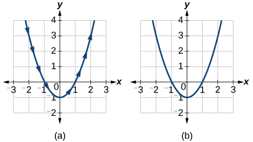
Analysis

The arrows indicate the direction in which the curve is generated. Notice the curve is identical to the curve of \(y=x^2−1\).

Exercise \(\PageIndex{1}\)

Construct a table of values and plot the parametric equations: \(x(t)=t−3\), \(y(t)=2t+4\); \(−1≤t≤2\).

Answer

\(t\)	\(x(t)\)	\(y(t)\)
\(-1\)	\(-4\)	\(2\)
\(0\)	\(-3\)	\(4\)
\(1\)	\(-2\)	\(6\)
\(2\)	\(-1\)	\(8\)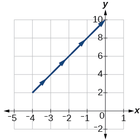

Figure \(\PageIndex{4}\)

Example \(\PageIndex{2}\): Finding a Pair of Parametric Equations

Find a pair of parametric equations that models the graph of \(y=1−x^2\), using the parameter \(x(t)=t\). Plot some points and sketch the graph.

Solution

If \(x(t)=t\) and we substitute \(t\) for \(x\) into the \(y\) equation, then \(y(t)=1−t^2\). Our pair of parametric equations is

\[\begin{align*} x(t) &=t \\ y(t) &= 1−t^2 \end{align*}\]

To graph the equations, first we construct a table of values like that in Table \(\PageIndex{2}\). We can choose values around \(t=0\), from \(t=−3\) to \(t=3\). The values in the \(x(t)\) column will be the same as those in the \(t\) column because \(x(t)=t\). Calculate values for the column \(y(t)\).

Table \(\PageIndex{2}\)

\(t)	\(x(t)=t\)	\(y(t)=1−t^2\)
\(−3\)	\(−3\)	\(y(−3)=1−{(−3)}^2=−8\)
\(−2\)	\(−2\)	\(y(−2)=1−{(−2)}^2=−3\)
\(−1\)	\(−1\)	\(y(−1)=1−{(−1)}^2=0\)
\(0\)	\(0\)	\(y(0)=1−0=1\)
\(1\)	\(1\)	\(y(1)=1−{(1)}^2=0\)
\(2\)	\(2\)	\(y(2)=1−{(2)}^2=−3\)
\(3\)	\(3\)	\(y(3)=1−{(3)}^2=−8\)

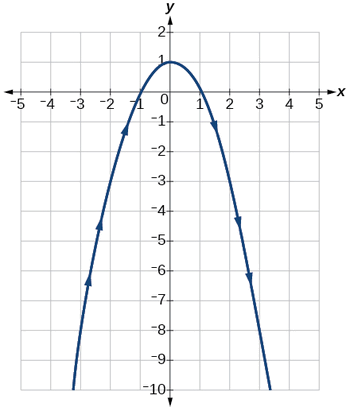
The graph of \(y=1−t^2\) is a parabola facing downward, as shown in Figure \(\PageIndex{5}\). We have mapped the curve over the interval \([−3, 3]\), shown as a solid line with arrows indicating the orientation of the curve according to \(t\). Orientation refers to the path traced along the curve in terms of increasing values of \(t\). As this parabola is symmetric with respect to the line \(x=0\), the values of \(x\) are reflected across the y-axis.

Figure \(\PageIndex{5}\)

Exercise \(\PageIndex{2}\)

Parameterize the curve given by \(x=y^3−2y\).

Answer

\(x(t)=t^3−2t\)

\(y(t)=t\)

Example \(\PageIndex{3}\): Finding Parametric Equations That Model Given Criteria

An object travels at a steady rate along a straight path \((−5, 3)\) to \((3, −1)\) in the same plane in four seconds. The coordinates are measured in meters. Find parametric equations for the position of the object.

Solution

The parametric equations are simple linear expressions, but we need to view this problem in a step-by-step fashion. Thex-value of the object starts at \(−5\) meters and goes to \(3\) meters. This means the distance \(x\) has changed by \(8\) meters in \(4\) seconds, which is a rate of \(\dfrac{8\space m}{4\space s}\), or \(2\space m/s\). We can write the x-coordinate as a linear function with respect to time as \(x(t)=2t−5\). In the linear function template \(y=mx+b\), \(2t=mx\) and \(−5=b\).

Similarly, the \(y\)-value of the object starts at \(3\) and goes to \(−1\), which is a change in the distance \(y\) of \(−4\) meters in \(4\) seconds, which is a rate of \(\dfrac{−4\space m}{4\space s}\), or \(−1\space m/s\). We can also write the y-coordinate as the linear function \(y(t)=−t+3\). Together, these are the parametric equations for the position of the object, where \(x\) and \(y\) are expressed in meters and \(t\) represents time:

\[\begin{align*} x(t) &= 2t−5 \\ y(t) &= −t+3 \end{align*}\]

Using these equations, we can build a table of values for \(t\), \(x\), and \(y\) (see Table \(\PageIndex{3}\)). In this example, we limited values of \(t\) to non-negative numbers. In general, any value of \(t\) can be used.

Table \(\PageIndex{3}\)

\(t\)	\(x(t)=2t−5\)	\(y(t)=−t+3\)
\(0\)	\(x=2(0)−5=−5\)	\(y=−(0)+3=3\)
\(1\)	\(x=2(1)−5=−3\)	\(y=−(1)+3=2\)
\(2\)	\(x=2(2)−5=−1\)	\(y=−(2)+3=1\)
\(3\)	\(x=2(3)−5=1\)	\(y=−(3)+3=0\)
\(4\)	\(x=2(4)−5=3\)	\(y=−(4)+3=−1\)

From this table, we can create three graphs, as shown in Figure \(\PageIndex{6}\).

Figure \(\PageIndex{6}\) : (a) A graph of \(x\) vs. \(t\), representing the horizontal position over time. (b) A graph of \(y\) vs. \(t\), representing the vertical position over time. (c) A graph of \(y\) vs. \(x\), representing the position of the object in the plane at time \(t\).

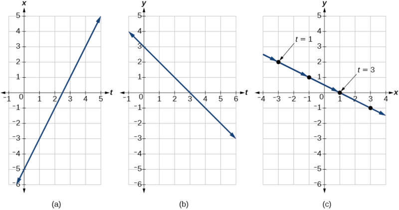
Analysis

Again, we see that, in Figure \(\PageIndex{6}\) (c), when the parameter represents time, we can indicate the movement of the object along the path with arrows.

Eliminating the Parameter

In many cases, we may have a pair of parametric equations but find that it is simpler to draw a curve if the equation involves only two variables, such as \(x\) and \(y\). Eliminating the parameter is a method that may make graphing some curves easier. However, if we are concerned with the mapping of the equation according to time, then it will be necessary to indicate the orientation of the curve as well. There are various methods for eliminating the parameter \(t\) from a set of parametric equations; not every method works for every type of equation. Here we will review the methods for the most common types of equations.

Eliminating the Parameter from Polynomial, Exponential, and Logarithmic Equations

For polynomial, exponential, or logarithmic equations expressed as two parametric equations, we choose the equation that is most easily manipulated and solve for \(t\). We substitute the resulting expression for \(t\) into the second equation. This gives one equation in \(x\) and \(y\).

Example \(\PageIndex{4}\): Eliminating the Parameter in Polynomials

Given \(x(t)=t^2+1\) and \(y(t)=2+t\), eliminate the parameter, and write the parametric equations as a Cartesian equation.

Solution

We will begin with the equation for \(y\) because the linear equation is easier to solve for \(t\).

\[\begin{align*} y &= 2+t \\ y−2 &=t \end{align*}\]

Next, substitute \(y−2\) for \(t\) in \(x(t)\).

\[\begin{align*} x &= t^2+1 \\ x &= {(y−2)}^2+1 \;\;\;\;\;\;\;\; \text{Substitute the expression for }t \text{ into }x. \\ x &= y^2−4y+4+1 \\ x &= y^2−4y+5 \\ x &= y^2−4y+5 \end{align*}\]

The Cartesian form is \(x=y^2−4y+5\).

Analysis

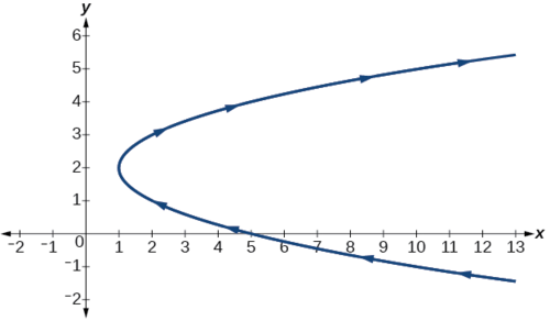
This is an equation for a parabola in which, in rectangular terms, \(x\) is dependent on \(y\). From the curve’s vertex at \((1,2)\), the graph sweeps out to the right. See Figure \(\PageIndex{7}\). In this section, we consider sets of equations given by the functions \(x(t)\) and \(y(t)\), where \(t\) is the independent variable of time. Notice, both \(x\) and \(y\) are functions of time; so in general \(y\) is not a function of \(x\).

Figure \(\PageIndex{7}\)

Exercise \(\PageIndex{3}\)

Given the equations below, eliminate the parameter and write as a rectangular equation for \(y\) as a function of \(x\).

\[\begin{align*} x(t) &= 2t^2+6 \\ y(t) &= 5−t \end{align*}\]

Answer

\(y=5−\sqrt{\frac{1}{2}x−3}\)

Example \(\PageIndex{5}\): Eliminating the Parameter in Exponential Equations

Eliminate the parameter and write as a Cartesian equation: \(x(t)=e^{−t}\) and \(y(t)=3e^t\),\(t>0\).

Solution

Isolate \(e^t\).

\[\begin{align*} x &=e^{−t} \\ e^t &= \dfrac{1}{x} \end{align*}\]

Substitute the expression into \(y(t)\).

\[\begin{align*} y &= 3e^t \\ y &= 3 \left(\dfrac{1}{x}\right) \\ y &= \dfrac{3}{x} \end{align*}\]

The Cartesian form is \(y=\dfrac{3}{x}\).

Analysis

The graph of the parametric equation is shown in Figure \(\PageIndex{8a}\). The domain is restricted to \(t>0\). The Cartesian equation, \(y=\dfrac{3}{x}\) is shown in Figure \(\PageIndex{8b}\) and has only one restriction on the domain, \(x≠0\).

Figure \(\PageIndex{8}\)

Example \(\PageIndex{6}\): Eliminating the Parameter in Logarithmic Equations

Eliminate the parameter and write as a Cartesian equation: \(x(t)=\sqrt{t}+2\) and \(y(t)=\log(t)\).

Solution

Solve the first equation for \(t\).

\[\begin{align*} x &= \sqrt{t}+2 \\ x−2 &= \sqrt{t} \\ {(x−2)}^2 &= t \;\;\;\;\;\;\;\; \text{Square both sides.} \end{align*}\]

Then, substitute the expression for \(t\) into the \(y\) equation.

\[\begin{align*} y &= \log(t) \\ y &= \log{(x−2)}^2 \end{align*}\]

The Cartesian form is \(y=\log{(x−2)}^2\).

Analysis

To be sure that the parametric equations are equivalent to the Cartesian equation, check the domains. The parametric equations restrict the domain on \(x=\sqrt{t}+2\) to \(t>0\); we restrict the domain on \(x\) to \(x>2\). The domain for the parametric equation \(y=\log(t)\) is restricted to \(t>0\); we limit the domain on \(y=\log{(x−2)}^2\) to \(x>2\).

Exercise \(\PageIndex{4}\)

Eliminate the parameter and write as a rectangular equation.

\[\begin{align*} x(t) &= t^2 \\ y(t) &= \ln t\text{, } t>0 \end{align*}\]

Answer

\(y=\ln \sqrt{x}\)

Eliminating the Parameter from Trigonometric Equations

Eliminating the parameter from trigonometric equations is a straightforward substitution. We can use a few of the familiar trigonometric identities and the Pythagorean Theorem.

First, we use the identities:

\[\begin{align*} x(t) &= a \cos t \\ y(t) &= b \sin t \end{align*}\]

Solving for \(\cos t\) and \(\sin t\), we have

\[\begin{align*} \dfrac{x}{a} &= \cos t \\ \dfrac{y}{b} &= \sin t \end{align*}\]

Then, use the Pythagorean Theorem:

\({\cos}^2 t+{\sin}^2 t=1\)

Substituting gives

\({\cos}^2 t+{\sin}^2 t={\left(\dfrac{x}{a}\right)}^2+{\left(\dfrac{y}{b}\right)}^2=1\)

Example \(\PageIndex{7}\): Eliminating the Parameter from a Pair of Trigonometric Parametric Equations

Eliminate the parameter from the given pair of trigonometric equations where \(0≤t≤2\pi\) and sketch the graph.

\[\begin{align*} x(t) &=4 \cos t \\ y(t) &=3 \sin t \end{align*}\]

Solution

Solving for \(\cos t\) and \(\sin t\), we have

\[\begin{align*} x &=4 \cos t \\ \dfrac{x}{4} &= \cos t \\ y &=3 \sin t \\ \dfrac{y}{3} &= \sin t \end{align*}\]

Next, use the Pythagorean identity and make the substitutions.

\[\begin{align*} {\cos}^2 t+{\sin}^2 t &= 1 \\ {\left(\dfrac{x}{4}\right)}^2+{\left(\dfrac{y}{3}\right)}^2 &=1 \\ \dfrac{x^2}{16}+\dfrac{y^2}{9} &=1 \end{align*}\]

The graph for the equation is shown in Figure \(\PageIndex{9}\) .

Figure \(\PageIndex{9}\)

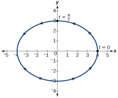
Analysis

Applying the general equations for conic sections (introduced in Analytic Geometry, we can identify \(\dfrac{x^2}{16}+\dfrac{y^2}{9}=1\) as an ellipse centered at \((0,0)\). Notice that when \(t=0\) the coordinates are \((4,0)\), and when \(t=\dfrac{\pi}{2}\) the coordinates are \((0,3)\). This shows the orientation of the curve with increasing values of \(t\).

Exercise \(\PageIndex{5}\)

Eliminate the parameter from the given pair of parametric equations and write as a Cartesian equation: \(x(t)=2 \cos t\) and \(y(t)=3 \sin t\).

Answer

\(\dfrac{x^2}{4}+\dfrac{y^2}{9}=1\)

Finding Cartesian Equations from Curves Defined Parametrically

When we are given a set of parametric equations and need to find an equivalent Cartesian equation, we are essentially “eliminating the parameter.” However, there are various methods we can use to rewrite a set of parametric equations as a Cartesian equation. The simplest method is to set one equation equal to the parameter, such as \(x(t)=t\). In this case, \(y(t)\) can be any expression. For example, consider the following pair of equations.

\[\begin{align*} x(t) &=t \\ y(t) &= t^2−3 \end{align*}\]

Rewriting this set of parametric equations is a matter of substituting \(x\) for \(t\). Thus, the Cartesian equation is \(y=x^2−3\).

Example \(\PageIndex{8}\): Finding a Cartesian Equation Using Alternate Methods

Use two different methods to find the Cartesian equation equivalent to the given set of parametric equations.

\[\begin{align*} x(t) &= 3t−2 \\ y(t) &= t+1 \end{align*}\]

Solution

Method 1. First, let’s solve the \(x\) equation for \(t\). Then we can substitute the result into the \(y\) equation.

\[\begin{align*} x &= 3t−2 \\ x+2 &= 3t \\ \dfrac{x+2}{3} &= t \end{align*}\]

Now substitute the expression for \(t\) into the \(y\) equation.

\[\begin{align*} y &= t+1 \\ y & = \left(\dfrac{x+2}{3}\right)+1 \\ y &= \dfrac{x}{3}+\dfrac{2}{3}+1 \\ y &= \dfrac{1}{3}x+\dfrac{5}{3} \end{align*}\]

Method 2. Solve the \(y\) equation for \(t\) and substitute this expression in the \(x\) equation.

\[\begin{align*} y &= t+1 \\ y−1 &=t \end{align*}\]

Make the substitution and then solve for \(y\).

\[\begin{align*} x &= 3(y−1)−2 \\ x &= 3y−3−2 \\ x &= 3y−5 \\ x+5 &= 3y \\ \dfrac{x+5}{3} &= y \\ y &= \dfrac{1}{3}x+\dfrac{5}{3} \end{align*}\]

Exercise \(\PageIndex{6}\)

Write the given parametric equations as a Cartesian equation: \(x(t)=t^3\) and \(y(t)=t^6\).

Answer

\(y=x^2\)

Finding Parametric Equations for Curves Defined by Rectangular Equations

Although we have just shown that there is only one way to interpret a set of parametric equations as a rectangular equation, there are multiple ways to interpret a rectangular equation as a set of parametric equations. Any strategy we may use to find the parametric equations is valid if it produces equivalency. In other words, if we choose an expression to represent \(x\), and then substitute it into the \(y\) equation, and it produces the same graph over the same domain as the rectangular equation, then the set of parametric equations is valid. If the domain becomes restricted in the set of parametric equations, and the function does not allow the same values for \(x\) as the domain of the rectangular equation, then the graphs will be different.

Example \(\PageIndex{9}\): Finding a Set of Parametric Equations for Curves Defined by Rectangular Equations

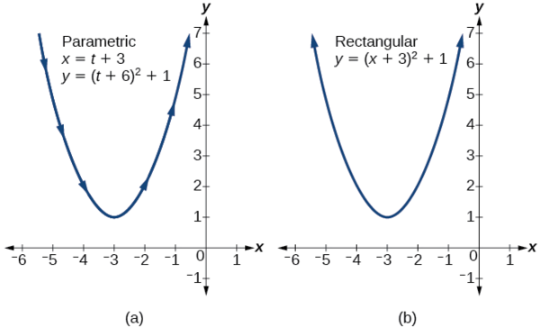
Find a set of equivalent parametric equations for \(y={(x+3)}^2+1\).

Solution

An obvious choice would be to let \(x(t)=t\). Then \(y(t)={(t+3)}^2+1\). But let’s try something more interesting. What if we let \(x=t+3\)? Then we have

\[\begin{align*} y &= {(x+3)}^2+1 \\ y &= {((t+3)+3)}^2+1 \\ y &= {(t+6)}^2+1 \end{align*}\]

The set of parametric equations is

\[\begin{align*} x(t) &= t+3 \\ y(t) &= {(t+6)}^2+1 \end{align*}\]

See Figure \(\PageIndex{10}\).

Figure \(\PageIndex{10}\)

Media

Access these online resources for additional instruction and practice with parametric equations.

• Introduction to Parametric Equations
• Converting Parametric Equations to Rectangular Form

Key Concepts

• Parameterizing a curve involves translating a rectangular equation in two variables, \(x\) and \(y\), into two equations in three variables, \(x\), \(y\), and \(t\). Often, more information is obtained from a set of parametric equations. See Example \(\PageIndex{1}\), Example \(\PageIndex{2}\), and Example \(\PageIndex{3}\).
• Sometimes equations are simpler to graph when written in rectangular form. By eliminating \(t\), an equation in \(x\) and \(y\) is the result.
• To eliminate \(t\), solve one of the equations for \(t\), and substitute the expression into the second equation. See Example \(\PageIndex{4}\), Example \(\PageIndex{5}\), Example \(\PageIndex{6}\), and Example \(\PageIndex{7}\).
• Finding the rectangular equation for a curve defined parametrically is basically the same as eliminating the parameter. Solve for \(t\) in one of the equations, and substitute the expression into the second equation. See Example \(\PageIndex{8}\).
• There are an infinite number of ways to choose a set of parametric equations for a curve defined as a rectangular equation.
• Find an expression for \(x\) such that the domain of the set of parametric equations remains the same as the original rectangular equation. See Example \(\PageIndex{9}\).

Contributors

• Jay Abramson (Arizona State University) with contributing authors. Textbook content produced by OpenStax College is licensed under a Creative Commons Attribution License 4.0 license. Download for free at https://openstax.org/details/books/precalculus.