
8.5: Clustering

( \newcommand{\kernel}{\mathrm{null}\,}\)
Watts (1999) and many others have noted that in large, real-world networks (of all kinds of things) there is often a structural pattern that seems somewhat paradoxical.
On one hand, in many large networks (like, for example, the Internet) the average geodesic distance between any two nodes is relatively short. The "6-degrees" of distance phenomenon is an example of this. So, most of the nodes in even very large networks may be fairly close to one another. The average distance between pairs of actors in large empirical networks are often much shorter than in random graphs of the same size.
On the other hand, most actors live in local neighborhoods where most others are also connected to one another. That is, in most large networks, a very large proportion of the total number of ties are highly "clustered" into local neighborhoods. That is, the density in local neighborhoods of large graphs tend to be much higher than we would expect for a random graph of the same size.
Most of the people we know may also know one another - seeming to locate us in a very narrow social world. Yet, at the same time, we can be at quite short distances to vast numbers of people that we don't know at all. The "small world" phenomenon - a combination of short average path lengths over the entire graph, coupled with a strong degree of "clique-like" local neighborhoods - seems to have evolved independently in many large networks.
We've already discussed one part of this phenomenon. The average geodesic distance between all actors in a graph gets at the idea of how close actors are together. The other part of the phenomenon is the tendency towards dense local neighborhoods, or what is now thought of as "clustering".
One common way of measuring the extent to which a graph displays clustering is to examine the local neighborhood of an actor (that is, all the actors who are directly connected to ego), and to calculate the density in this neighborhood (leaving out ego). After doing this for all actors in the whole network, we can characterize the degree of clustering as an average of all the neighborhoods.
Figure 8.8 shows the output of Network>Cohesion>Clustering Coefficient as applied to the Knoke information network.
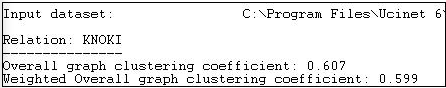
Figure 8.8: Network>Cohesion>Clustering Coefficient of Knoke information network
Two alternative measures are presented. The "overall" graph clustering coefficient is simply the average of the densities of the neighborhoods of all of the actors. The "weighted" version gives weight to the neighborhood densities proportional to their size; that is, actors with larger neighborhoods get more weight in computing the average density. Since larger graphs are generally (but not necessarily) less dense than smaller ones, the weighted average neighborhood density (or clustering coefficient) is usually less than the unweighted version. In our example, we see that all of the actors are surrounded by local neighborhoods that are fairly dense - our organizations can be seen as embedded in dense local neighborhoods to a fairly high degree. Lest we over-interpret, we must remember that the overall density of the entire graph in this population is rather high (0.54). So, the density of local neighborhoods is not really much higher than the density of the whole graph. In assessing the degree of clustering, it is usually wise to compare the cluster coefficient to the overall density.
We can also examine the densities of the neighborhoods of each actor, as is shown in Figure 8.9.
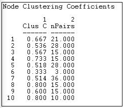
Figure 8.9: Node level clustering coefficients for Knoke information network
The sizes of each actor's neighborhood is reflected in the number of pairs of actors in it. Actor 6, for example, has three neighbors, and hence three possible ties. Of these, only one is present - so actor 6 is not highly clustered. Actor 8, on the other hand, is in a slightly larger neighborhood (6 neighbors, and hence 15 pairs of neighbors), but 80% of all the possible ties among these neighbors are present. Actors 8 and 10 are embedded in highly clustered neighbors.