9.4: Structural Holes
- Page ID
- 7703
\( \newcommand{\vecs}[1]{\overset { \scriptstyle \rightharpoonup} {\mathbf{#1}} } \)
\( \newcommand{\vecd}[1]{\overset{-\!-\!\rightharpoonup}{\vphantom{a}\smash {#1}}} \)
\( \newcommand{\id}{\mathrm{id}}\) \( \newcommand{\Span}{\mathrm{span}}\)
( \newcommand{\kernel}{\mathrm{null}\,}\) \( \newcommand{\range}{\mathrm{range}\,}\)
\( \newcommand{\RealPart}{\mathrm{Re}}\) \( \newcommand{\ImaginaryPart}{\mathrm{Im}}\)
\( \newcommand{\Argument}{\mathrm{Arg}}\) \( \newcommand{\norm}[1]{\| #1 \|}\)
\( \newcommand{\inner}[2]{\langle #1, #2 \rangle}\)
\( \newcommand{\Span}{\mathrm{span}}\)
\( \newcommand{\id}{\mathrm{id}}\)
\( \newcommand{\Span}{\mathrm{span}}\)
\( \newcommand{\kernel}{\mathrm{null}\,}\)
\( \newcommand{\range}{\mathrm{range}\,}\)
\( \newcommand{\RealPart}{\mathrm{Re}}\)
\( \newcommand{\ImaginaryPart}{\mathrm{Im}}\)
\( \newcommand{\Argument}{\mathrm{Arg}}\)
\( \newcommand{\norm}[1]{\| #1 \|}\)
\( \newcommand{\inner}[2]{\langle #1, #2 \rangle}\)
\( \newcommand{\Span}{\mathrm{span}}\) \( \newcommand{\AA}{\unicode[.8,0]{x212B}}\)
\( \newcommand{\vectorA}[1]{\vec{#1}} % arrow\)
\( \newcommand{\vectorAt}[1]{\vec{\text{#1}}} % arrow\)
\( \newcommand{\vectorB}[1]{\overset { \scriptstyle \rightharpoonup} {\mathbf{#1}} } \)
\( \newcommand{\vectorC}[1]{\textbf{#1}} \)
\( \newcommand{\vectorD}[1]{\overrightarrow{#1}} \)
\( \newcommand{\vectorDt}[1]{\overrightarrow{\text{#1}}} \)
\( \newcommand{\vectE}[1]{\overset{-\!-\!\rightharpoonup}{\vphantom{a}\smash{\mathbf {#1}}}} \)
\( \newcommand{\vecs}[1]{\overset { \scriptstyle \rightharpoonup} {\mathbf{#1}} } \)
\( \newcommand{\vecd}[1]{\overset{-\!-\!\rightharpoonup}{\vphantom{a}\smash {#1}}} \)
\(\newcommand{\avec}{\mathbf a}\) \(\newcommand{\bvec}{\mathbf b}\) \(\newcommand{\cvec}{\mathbf c}\) \(\newcommand{\dvec}{\mathbf d}\) \(\newcommand{\dtil}{\widetilde{\mathbf d}}\) \(\newcommand{\evec}{\mathbf e}\) \(\newcommand{\fvec}{\mathbf f}\) \(\newcommand{\nvec}{\mathbf n}\) \(\newcommand{\pvec}{\mathbf p}\) \(\newcommand{\qvec}{\mathbf q}\) \(\newcommand{\svec}{\mathbf s}\) \(\newcommand{\tvec}{\mathbf t}\) \(\newcommand{\uvec}{\mathbf u}\) \(\newcommand{\vvec}{\mathbf v}\) \(\newcommand{\wvec}{\mathbf w}\) \(\newcommand{\xvec}{\mathbf x}\) \(\newcommand{\yvec}{\mathbf y}\) \(\newcommand{\zvec}{\mathbf z}\) \(\newcommand{\rvec}{\mathbf r}\) \(\newcommand{\mvec}{\mathbf m}\) \(\newcommand{\zerovec}{\mathbf 0}\) \(\newcommand{\onevec}{\mathbf 1}\) \(\newcommand{\real}{\mathbb R}\) \(\newcommand{\twovec}[2]{\left[\begin{array}{r}#1 \\ #2 \end{array}\right]}\) \(\newcommand{\ctwovec}[2]{\left[\begin{array}{c}#1 \\ #2 \end{array}\right]}\) \(\newcommand{\threevec}[3]{\left[\begin{array}{r}#1 \\ #2 \\ #3 \end{array}\right]}\) \(\newcommand{\cthreevec}[3]{\left[\begin{array}{c}#1 \\ #2 \\ #3 \end{array}\right]}\) \(\newcommand{\fourvec}[4]{\left[\begin{array}{r}#1 \\ #2 \\ #3 \\ #4 \end{array}\right]}\) \(\newcommand{\cfourvec}[4]{\left[\begin{array}{c}#1 \\ #2 \\ #3 \\ #4 \end{array}\right]}\) \(\newcommand{\fivevec}[5]{\left[\begin{array}{r}#1 \\ #2 \\ #3 \\ #4 \\ #5 \\ \end{array}\right]}\) \(\newcommand{\cfivevec}[5]{\left[\begin{array}{c}#1 \\ #2 \\ #3 \\ #4 \\ #5 \\ \end{array}\right]}\) \(\newcommand{\mattwo}[4]{\left[\begin{array}{rr}#1 \amp #2 \\ #3 \amp #4 \\ \end{array}\right]}\) \(\newcommand{\laspan}[1]{\text{Span}\{#1\}}\) \(\newcommand{\bcal}{\cal B}\) \(\newcommand{\ccal}{\cal C}\) \(\newcommand{\scal}{\cal S}\) \(\newcommand{\wcal}{\cal W}\) \(\newcommand{\ecal}{\cal E}\) \(\newcommand{\coords}[2]{\left\{#1\right\}_{#2}}\) \(\newcommand{\gray}[1]{\color{gray}{#1}}\) \(\newcommand{\lgray}[1]{\color{lightgray}{#1}}\) \(\newcommand{\rank}{\operatorname{rank}}\) \(\newcommand{\row}{\text{Row}}\) \(\newcommand{\col}{\text{Col}}\) \(\renewcommand{\row}{\text{Row}}\) \(\newcommand{\nul}{\text{Nul}}\) \(\newcommand{\var}{\text{Var}}\) \(\newcommand{\corr}{\text{corr}}\) \(\newcommand{\len}[1]{\left|#1\right|}\) \(\newcommand{\bbar}{\overline{\bvec}}\) \(\newcommand{\bhat}{\widehat{\bvec}}\) \(\newcommand{\bperp}{\bvec^\perp}\) \(\newcommand{\xhat}{\widehat{\xvec}}\) \(\newcommand{\vhat}{\widehat{\vvec}}\) \(\newcommand{\uhat}{\widehat{\uvec}}\) \(\newcommand{\what}{\widehat{\wvec}}\) \(\newcommand{\Sighat}{\widehat{\Sigma}}\) \(\newcommand{\lt}{<}\) \(\newcommand{\gt}{>}\) \(\newcommand{\amp}{&}\) \(\definecolor{fillinmathshade}{gray}{0.9}\)In several important works, Ronald Burt coined and popularized the term "structural holes" to refer to some very important aspects of positional advantage/disadvantage of individuals that result from how they are embedded in neighborhoods. Burt's formalization of these ideas, and his development of a number of measures (including the computer program Structure, that provides these measures and other tools) has facilitated a great deal of further thinking about how and why the ways that an actor is connected affect their constraints and opportunities, and hence their behavior.
The basic idea is simple, as good ideas often are.
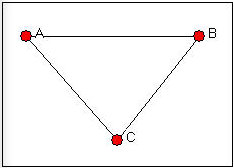
Imagine a network of three actors (A, B, and C), in which each is connected to each of the others, as in Figure 9.5.

Figure 9.5: Three actor network with no structural holes
Let's focus on actor A (of course, in this case, the situations of B and C are identical in this particular network). Suppose that actor A wanted to influence or exchange with another actor. Assume that both B and C may have some interest in interacting or exchanging, as well. Actor A will not be in a strong bargaining position in this network, because both of A's potential exchange partners (B and C) have alternatives to treating with A; they could isolate A, and exchange with one another.
Now imagine that we open a "structural hole" between actors B and C, as in Figure 9.6. That is, a relation or tie is "absent" such that B and C cannot exchange (perhaps they are not aware of one another, or there are very high transaction costs involved in forming a tie).

Figure 9.6: Three actor network with a structural hole
In this situation, actor A has an advantaged position as a direct result of the "structural hole" between actors B and C. Actor A has two alternative exchange partners; actors B and C have only one choice, if they choose to (or must) enter into an exchange.
Real networks, of course, usually have more actors. But, as networks grow in size, they tend to become less dense (how many relations can each actor support?). As density decreases, more "structural holes" are likely to open in the "social fabric". These holes, and how and where they are distributed can be a source of inequality (in both the strict mathematical sense and the sociological sense) among actors embedded in networks.
Network>Ego Networks>Structural Holes examines the position of each actor in their neighborhood for the presence of structural holes. A number of measures (most proposed by Burt) that describe various aspects of the advantage or disadvantage of the actor are also computed. Figure 9.7 shows a typical dialog box; we're looking at the Knoke information network again.

Figure 9.7: Network>Ego Networks>Structural Holes dialog
Measures related to structural holes can be computed on both valued and binary data. The normal practice in sociological research has been to use binary (a relation is present or not). Interpretation of the measures becomes quite difficult with valued data (at least I find it difficult). As an alternative to losing the information that valued data may provide, the input data could be dichotomized (Transform>Dichotomize) at various levels of strength. The structural holes measures may be computed for either directed or undirected data - and the interpretation, of course, depends on which is used. Here, we've used the directed binary data. Three output arrays are produced, and can be saved as separate files (or not, as the output reports all three).
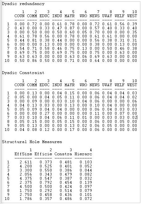
The results are shown in Figure 9.8, and need a bit of explanation.

Figure 9.8: Structural holes results for the Knoke information exchange network
- Dyadic redundancy means that ego's tie to alter is "redundant". If A is tied to both B and C, and B is tied to C (as in Figure 9.5), A's tie to B is redundant, because A can influence B by way of C. The dyadic redundancy measure calculates, for each actor in ego's neighborhood, how many of the other actors in the neighborhood are also tied to the other. The larger the proportion of others in the neighborhood who are tied to a give "alter", the more "redundant" is ego's direct tie. In the example, we see that actor 1's (COUN) tie to actor 2 (COMM) is largely redundant, as \(72\%\) of ego's other neighbors also have ties with COMM. Actors that display high dyadic redundancy are actors who are embedded in local neighborhoods where there are few structural holes.
- Dyadic constraint is a measure that indexes the extent to which the relationship between ego and each of the alters in ego's neighborhood "constrains" ego. A full description is given in Burt's 1992 monograph, and the construction of the measure is somewhat complex. At the core though, A is constrained by its relationship with B to the extent that A does not have many alternatives (has few other ties except that to B), and A's other alternatives are also tied to B. If A has few alternatives to exchanging with B, and if those alternative exchange partners are also tied to B, then B is likely to constrain A's behavior. In our example constraint measures are not very large, as most actors have several ties. COMM and MAYR are, however, exerting considerable numbers of ties, and many of the actors to whom they are tied do not have many independent sources of information.
- Effective size of the network (EffSize) is the number of alters that ego has, minus the average number of ties that each alter has to other alters. Suppose that A has ties to three other actors. Suppose that none of these three has ties to any of the others. The effective size of ego's network is three. Alternatively, suppose that A has ties to three others, and that all of the others are tied to one another. A's network size is three, but the ties are "redundant" because A can reach all three neighbors by reaching any one of them. The average degree of the others in this case is 2 (each alter is tied to two other alters). So, the effective size of the network is its actual size (3), reduced by its redundancy (2), to yield an effective size of 1.
- Efficiency (Efficie) norms the effective size of ego's network by its actual size. That is, what proportion of ego's ties to its neighborhood are "non-redundant". The effective size of ego's network may tell us something about ego's total impact; efficiency tells us how much impact ego is getting for each unit invested in using ties. An actor can be effective without being efficient; and an actor can be efficient without being effective.
- Constraint (Constra) is a summary measure that taps the extent to which ego's connections are to others who are connected to one another. If ego's potential trading partners all have one another as potential trading partners, ego is highly constrained. If ego's partners do not have other alternatives in the neighborhood, they cannot constrain ego's behavior. The logic is pretty simple, but the measure itself is not. It would be good to take a look at Burt's 1992 Structural Holes. The idea of constraint is an important one because it points out that actors who have many ties to others may actually lose freedom of action rather than gain it - depending on the relationships among the other actors.
- Hierarchy (Hierarc) is another quite complex measure that describes the nature of the constraint on ego. If the total constraint on ego is concentrated in a single other actor, the hierarchy measure will have a higher value. If the constraint results more equally from multiple actors in ego's neighborhood, hierarchy will be less. The hierarchy measure, in itself, does not assess the degree of constraint. But, among whatever constraint there is on ego, it measures the important property of dependency - inequality in the distribution of constraints on ego across the alters in its neighborhood.


