18.3: Comparing Two Relations for the Same Set of Actors
( \newcommand{\kernel}{\mathrm{null}\,}\)
The basic question of bivariate descriptive statistics applied to variables is whether scores on one attribute align (co-vary, correlate) with scores on another attribute, when compared across cases. The basic question of bivariate analysis of network data is whether the pattern of ties for one relation among a set of actors aligns with the pattern of ties for another relation among the same actors. That is, do the relations correlate?
Three of the most common tools for bivariate analysis of attributes can also be applied to the bivariate analysis of relations:
Does the central tendency of one relation differ significantly from the central tendency of another? For example, if we had two networks that described the military and the economic ties among nations, which has the higher density? Are military or are economic ties more prevalent? This kind of question is analogous to the test for the difference between means in paired or repeated-measures attribute analysis.
Is there a correlation between the ties that are present in one network, and the ties that are present in another? For example, are pairs of nations that have political alliances more likely to have high volumes of economic trade? This kind of question is analogous to the correlation between the scores on two variables in attribute analysis.
If we know that a relation of one type exists between two actors, how much does this increase (or decrease) the likelihood that a relation of another type exists between them? For example, what is the effect of a one dollar increase in the volume of trade between two nations on the volume of tourism flowing between the two nations? This kind of question is analogous to the regression of one variable on another in attribute analysis.
Hypotheses About Two Paired Means or Densities
In the section above on univariate statistics for networks, we noted that the density of the information exchange matrix for the Knoke bureaucracies appeared to be higher than the density of the monetary exchange matrix. That is, the mean or density of one relation among a set of actors appears to be different from the mean or density of another relation among the same actors.
Network>Compare densities>Paired (same node) compares the densities of two relations for the same actors, and calculates estimated standard errors to test differences by bootstrap methods. When both relations are binary, this is a test for differences in the probability of a tie of one type and the probability of a tie of another type. When both relations are valued, this is a test for a difference in the mean tie strengths of the two relations.
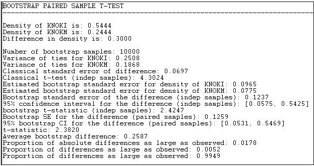
Let's perform this test on the information and money exchange relations in the Knoke data, as shown in Figure 18.7.

Figure 18.7: Test for the difference of density in the Knoke information and money exchange relations
Results for both the standard approach and the bootstrap approach (this time, we ran 10,000 sub-samples) are reported in the output. The difference between means (or proportions, or densities) is 0.3000. The standard error of the difference by the classical method is 0.0697; the standard error by bootstrap estimate is 0.1237. The conventional approach greatly underestimates the true sampling variability, and gives a result that is too optimistic in rejecting the null hypothesis that the two densities are the same.
By the bootstrap method, we can see that there is a two-tailed probability of 0.0178. If we had a prior alternative hypothesis about the direction of the difference, we could use the one-tailed p level of 0.0052. So, we can conclude with great confidence that the density of information ties among organizations is greater than the density of monetary ties. That is, the observed difference would arise very rarely by chance in random samples drawn from these networks.
Correlation Between Two Networks with the Same Actors
If there is a tie between two particular actors in one relation, is there likely to be a tie between them in another relation? If two actors have a strong tie of one type, are they also likely to have a strong tie of another?
When we have information about multiple relations among the same sets of actors, it is often of considerable interest whether the probability (or strength) of a tie of one type is related to the probability (or strength) of another. Consider the Knoke information and money ties. If organizations exchange information, this may create a sense of trust, making monetary exchange relations more likely; or, if they exchange money, this may facilitate more open communications. That is, we might hypothesize that the matrix of information relations would be positively correlated with the matrix of monetary relations - pairs that engage in one type of exchange are more likely to engage in the other. Alternatively, it might be that the relations are complementary: money flows in one direction, information in the other (a negative correlation). Or, it may be that the two relations have nothing to do with one another (no correlation).
Tools>Testing Hypotheses>Dyadic (QAP)>QAP Correlation calculates measures of nominal, ordinal, and interval association between the relations in two matrices, and uses quadratic assignment procedures to develop standard errors to test for the significance of association. Figure 18.8 shows the results for the correlation between the Knoke information and monetary exchange networks.

Figure 18.8: Association between Knoke information and Knoke monetary networks by QAP correlation
The first column shows the values of five alternative measures of association. The Pearson correlation is a standard measure when both matrices have valued relations measured at the interval level. Gamma would be a reasonable choice if one or both relations were measured on an ordinal scale. Simple matching and the Jaccard coefficient are reasonable measures when both relations are binary; the Hamming distance is a measure of dissimilarity or distance between the scores in one matrix and the scores in the other (it is the number of values that differ, element-wise, from one matrix to the other).
The third column (Avg) shows the average value of the measure of association across a large number of trials in which the rows and columns of the two matrices have been randomly permuted. That is, what would the correlation (or other measure) be, on the average, if we matched random actors? The idea of the "Quadratic Assignment Procedure" is to identify the value of the measure of association when their really isn't any systematic connection between the two relations. This value, as you can see, is not necessarily zero -- because different measures of association will have limited ranges of values based on the distributions of scores in the two matrices. We note, for example, that there is an observed simple matching of 0.456 (i.e. if there is a 1 in a cell in matrix one, there is a 45.6% chance that there will be a 1 in the corresponding cell of matrix two). This would seem to indicate association. But, because of the density of the two matrices, matching randomly re-arranged matrices will display an average matching of .475. So the observed measure differs hardly at all from a random result.
To test the hypothesis that there is association, we look at the proportion of random trials that would generate a coefficient as large as (or as small as, depending on the measure) the statistic actually observed. These figures are reported (from the random permutation trials) in the columns labeled "P(large)" and "P(small)." The appropriate one of these values to test the null hypothesis of no association is shown in the column "Signif."
Network Regression
Rather than correlating one relation with another, we may wish to predict one relation knowing the other. That is, rather than symmetric association between the relations, we may wish to examine asymmetric association. The standard tool for this question is linear regression, and the approach may be extended to using more than one independent variable.
Suppose, for example, that we wanted to see if we could predict which of the Knoke bureaucracies sent information to which others. We can treat the information exchange network as our "dependent" network (with N = 90).
We might hypothesize that the presence of a money tie from one organization to another would increase the likelihood of an information tie (of course, from the previous section, we know this isn't empirically supported!). Furthermore, we might hypothesize that institutionally similar organizations would be more likely to exchange information. So, we have created another 10 by 10 matrix, coding each element to be a "1" if both organizations in the dyad are governmental bodies, or both are non-governmental bodies, and "0" if they are of mixed types.
We can now perform a standard multiple regression analysis by regressing each element in the information network on its corresponding elements in the monetary network and the government institution network. To estimate standard errors for R-squared and for the regression coefficients, we can use quadratic assignment. We will run many trials with the rows and columns in the dependent matrix randomly shuffled, and recover the R-square and regression coefficients from these runs. These are then used to assemble empirical sampling distributions to estimate standard errors under the hypothesis of no association.
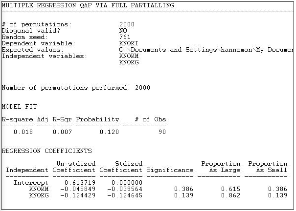
Version 6.81 of UCINET offers four alternative methods for Tools>Testing Hypotheses>Dyadic (QAP)>QAP Regression. Figure 18.9 shows the results of the "full partialling" method.

Figure 18.9: QAP regression of information ties on money ties and governmental status by full partialling method
The descriptive statistics and measure of goodness of fit are standard multiple regression results -- except, of course, that we are looking at predicting relations between actors, not the attributes of actors.
The model R-square (0.018) indicates that knowing whether one organization sends money to another, and whether the two organizations are institutionally similar reduces uncertainty in predicting an information tie by only about 2%. The significance level (by the QAP method) is 0.120. Usually, we would conclude that we cannot be sure the observed result is non-random.
Since the dependent matrix in this example is binary, the regression equation is interpretable as a linear probability model (one might want to consider logit or probit models -- but UCINET does not provide these). The intercept indicates that, if two organizations are not of the same institutional type, and one does not send money to the other, the probability that one sends information to the other is 0.61. If one organization does send money to the other, this reduces the probability of an information link by 0.046. If the two organizations are of the same institutional type, the probability of information sending is reduced by 0.124.
Using the QAP method, however, none of these effects are different from zero at conventional (e.g. p < 0.05) levels. The results are interesting - they suggest that monetary and informational linkages are, if anything, alternative rather than re-enforcing ties, and that institutionally similar organizations are less likely to communicate. But, we shouldn't take these apparent patterns seriously, because they could appear quite frequently simply by random permutation of the cases.
The tools in the this section are very useful for examining how multiplex relations among a set of actors "go together." These tools can often be helpful additions to some of the tools for working with multiplex data that we examined in chapter 16.


