18.4: Explaining Attributes of Networked Actors
- Page ID
- 7764
In the previous section we examined methods for testing differences and association among whole networks. That is, studying the macro-patterns of how an actor's position in one network might be associated with their position in another.
We are often interested in micro questions, as well. For example: does an actor's gender affect their between-ness centrality? This question relates an attribute (gender) to a measure of the actor's position in a network (between-ness centrality). We might be interested in the relationship between two (or more) aspects of actor's positions. For example: how much of the variation in actor's between-ness centrality can be explained by their out-degree and the number of cliques that they belong to? We might even be interested in the relationship between two individual attributes among a set of actors who are connected in a network. For example, in a school classroom, is there an association between actor's gender and their academic achievement?
In all of these cases we are focusing on variables that describe individual nodes. These variables may be either non-relational attributes (like gender), or variables that describe some aspect of an individual's relational position (like between-ness). In most cases, standard statistical tools for the analysis of variables can be applied to describe differences and associations.
But, standard statistical tools for the analysis of variables cannot be applied to inferential questions -- hypothesis or significance tests, because the individuals we are examining are not independent observations drawn at random from some large population. Instead of applying the normal formulas (i.e. those built into statistical software packages and discussed in most basic statistics texts), we need to use other methods to get more correct estimates of the reliability and stability of estimates (i.e. standard errors). The "boot-strapping" approach (estimating the variation of estimates of the parameter of interest from large numbers of random sub-samples of actors) can be applied in some cases; in other cases, the idea of random permutation can be applied to generate correct standard errors.
Hypotheses About the Means of Two Groups
Suppose we had the notion that private-for-profit organizations were less likely to actively engage in sharing information with others in their field than were government organizations. We would like to test this hypothesis by comparing the average out-degree of governmental and non-governmental actors in one organizational field.
Using the Knoke information exchange network, we've run Network>Centrality>Degree, and saved the results in the output file "FreemanDegree" as a UCINET dataset. We've also used Data>Spreadsheets>Matrix to create a UCINET attribute file "knokegovt" that has a single column dummy code (1 = governmental organization, 0 = non-governmental organization).
Let's perform a simple two-sample t-test to determine if the mean degree centrality of government organizations is lower than the mean degree centrality of non-government organizations. Figure 18.10 shows the dialog for Tools>Testing Hypotheses>Node-level>T-Test to set up this test.

Figure 18.10: Dialog for Tools>Testing Hypotheses>Node-level>T-Test
Since we are working with individual nodes as observations, the data are located in a column (or, sometimes, a row) of one or more files. Note how the file names (selected by browsing, or typed) and the columns within the file are entered in the dialog. The normed Freeman degree centrality measure happens to be located in the second column of its file; there is only one vector (column) in the file that we created to code government/non-government organizations.
For this test, we have selected the default of 10,000 trials to create the permutation-based sampling distribution of the difference between the two means. For each of these trials, the scores on normed Freeman degree centralization are randomly permuted (that is, randomly assigned to government or non-government, proportional to the number of each type.) The standard deviation of this distribution based on random trials becomes the estimated standard error for our test. Figure 18.11 shows the results.

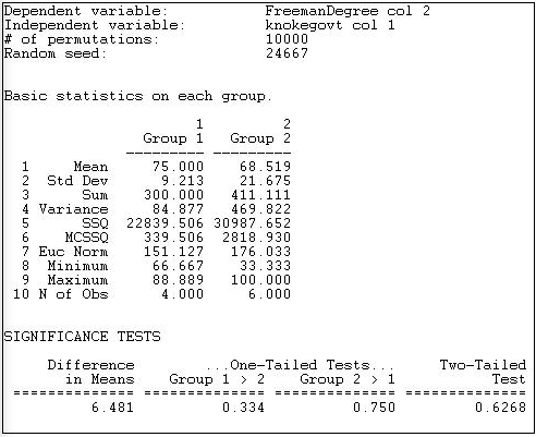
Figure 18.11: Test for difference in mean normed degree centrality of Knoke government and non-government organizations
The output first reports basic descriptive statistics for each group. The group numbers are assigned according to the order of the cases in the file containing the independent variable. In our example, the first node was COUN, a government organization; so, government became "Group 1" and non-government became "Group 2."
We see that the average normed degree centrality of government organizations (75) is 6.481 units higher than the average normed degree centrality of non-governmental organizations (68.519). This would seem to support our hypothesis; but tests of statistical significance urge considerable caution. Differences as large as 6.481 in favor of government organizations happen 33.4% of the time in random trials -- so we would be taking an unacceptable risk of being wrong if we concluded that the data were consistent with our research hypothesis.
UCINET does not print the estimated standard error, or the values of the conventional two-group t-test.
Hypotheses About the Means of Multiple Groups
The approach to estimating difference between the means of two groups discussed in the previous section can be extended to multiple groups with one-way analysis of variance (ANOVA). The procedure Tools>Testing Hypotheses>Node-level>Anova provides the regular OLS approach to estimating differences in group means. Because our observations are not independent, the procedure of estimating standard errors by random replications is also applied.
Suppose we divided the 23 large donors to California political campaigns into three groups, and have coded a single column vector in a UCINET attribute file. We've coded each donor as falling into one of three groups: "others," "capitalists," or "workers."
If we examine the network of connections among donors (defined by co-participating in the same campaigns), we anticipate that the worker's groups will display higher eigenvector centrality than donors in the other groups. That is, we anticipate that the "left" interest groups will display considerable interconnection, and -- on the average -- have members that are more connected to highly connected others than is true for the capitalist and other groups. We've calculated eigenvector centrality using Network>Centrality>Eigenvector, and stored the results in another UCINET attribute file.
The dialog for Tools>Testing Hypotheses>Node-level>Anova looks very much like Tools>Testing Hypotheses>Node-level>T-test, so we won't display it. The results of our analysis are shown as figure 18.12.

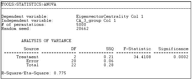
Figure 18.12: One-way ANOVA of eigenvector centrality of California political donors, with permutation-based standard errors and tests
The mean eigenvector centrality of the eight "other" donors is .125. For the seven "capitalists" it is 0.106, and for the seven "workers" groups it is 0.323 (calculated elsewhere). The differences among these means is highly significant (F = 34.4 with 2 d.f. and p = 0.0002). The differences in group means account for 78% of the total variance in eigenvector centrality scores among the donors.
Regressing Position on Attributes
Where the attribute of actors that we are interested in explaining or predicting is measured at the interval level, and one or more of our predictors are also at the interval level, multiple linear regression is a common approach. Tools>Testing Hypotheses>Node-level>Regression will compute basic linear multiple regression statistics by OLS, and estimate standard errors and significance using the random permutations method for constructing sampling distributions of R-squared and slope coefficients.
Let's continue the example in the previous section. Our dependent attribute, as before, is the eigenvector centrality of the individual political donors. This time, we will use three independent vectors, which we have constructed using Data>Spreadsheets>Matrix, as shown in figure 18.13.

Figure 18.13: Construction of independent vectors for multiple linear regression
Two dummy variables have been constructed to indicate whether each donor is a member of the "capitalist" or the "worker" group. The omitted category ("other") will serve as the intercept/reference category. POSCOAL is the mean number of times that each donor participates on the same side of issues with other donors (a negative score indicates opposition to other donors).
Substantively, we are trying to find out whether the "workers" higher eigenvector centrality (observed in the section above) is simply a function of higher rates of participation in coalitions, or whether the workers have better connected allies -- independent of high participation.
Figure 18.14 shows the dialog to specify the dependent and the multiple independent vectors.

Figure 18.14: Dialog for Tools>Testing Hypotheses>Node-level>Regression
Note that all of the independent variables need to be entered into a single data set (with multiple columns). All of the basic regression statistics can be saved as output, for use in graphics or further analysis. Figure 18.15 shows the result of the multiple regression estimation.

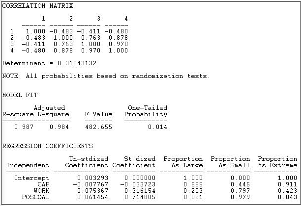
Figure 18.15: Multiple regression of eigenvector centrality with permutation based significance tests
The correlation matrix shows a very high collinearity between being in the workers group (variable 3) and participation in coalitions (variable 4). This suggests that it may be difficult to separate effects of simple participation from those of being a workers interest group.
The R-squared is very high for this simple model (.987), and highly significant using permutation tests ( p = 0.014).
Controlling for total coalition participation, capitalist interests are likely to have slightly lower eigenvector centrality than others (-0.0078), but this is not significant (p = 0.555). Workers groups do appear to have higher eigenvector centrality, even controlling for total coalition participation (0.075), but this tendency may be a random result (a one-tailed significance is only p = 0.102). The higher the rate of participation in coalitions (POSCOAL), the greater the eigenvector centrality of actors (0.0615, p = 0.021), regardless of which type of interest is being represented.
As before, the coefficients are generated by standard OLS linear modeling techniques, and are based on comparing scores on independent and dependent attributes of individual actors. What differs here is the recognition that the actors are not independent, so that estimation of standard errors by simulation, rather than by standard formula, is necessary.
The t-test, ANOVA, and regression approaches discussed in this section are all calculated at the micro, or individual actor level. The measures that are analyzed as independent and dependent may be either relational or non-relational. That is, we could be interested in predicting and testing hypotheses about actors non-relational attributes (e.g. their income) using a mix of relational (e.g. centrality) and non-relational (e.g. gender) attributes. We could be interested in predicting a relational attribute of actors (e.g. centrality) using a mix of relational and non-relational independent variables.
The examples illustrate how relational and non-relational attributes of actors can be analyzed using common statistical techniques. The key thing to remember, though, is that the observations are not independent (since all the actors are members of the same network). Because of this, direct estimation of the sampling distributions and resulting inferential statistics is needed -- standard, basic statistical software will not give correct answers.


