
7.4: Asymptotic Behavior of Continuous-Time Linear Dynamical Systems
- Page ID
- 7806

\( \newcommand{\vecs}[1]{\overset { \scriptstyle \rightharpoonup} {\mathbf{#1}} } \)
\( \newcommand{\vecd}[1]{\overset{-\!-\!\rightharpoonup}{\vphantom{a}\smash {#1}}} \)
\( \newcommand{\id}{\mathrm{id}}\) \( \newcommand{\Span}{\mathrm{span}}\)
( \newcommand{\kernel}{\mathrm{null}\,}\) \( \newcommand{\range}{\mathrm{range}\,}\)
\( \newcommand{\RealPart}{\mathrm{Re}}\) \( \newcommand{\ImaginaryPart}{\mathrm{Im}}\)
\( \newcommand{\Argument}{\mathrm{Arg}}\) \( \newcommand{\norm}[1]{\| #1 \|}\)
\( \newcommand{\inner}[2]{\langle #1, #2 \rangle}\)
\( \newcommand{\Span}{\mathrm{span}}\)
\( \newcommand{\id}{\mathrm{id}}\)
\( \newcommand{\Span}{\mathrm{span}}\)
\( \newcommand{\kernel}{\mathrm{null}\,}\)
\( \newcommand{\range}{\mathrm{range}\,}\)
\( \newcommand{\RealPart}{\mathrm{Re}}\)
\( \newcommand{\ImaginaryPart}{\mathrm{Im}}\)
\( \newcommand{\Argument}{\mathrm{Arg}}\)
\( \newcommand{\norm}[1]{\| #1 \|}\)
\( \newcommand{\inner}[2]{\langle #1, #2 \rangle}\)
\( \newcommand{\Span}{\mathrm{span}}\) \( \newcommand{\AA}{\unicode[.8,0]{x212B}}\)
\( \newcommand{\vectorA}[1]{\vec{#1}} % arrow\)
\( \newcommand{\vectorAt}[1]{\vec{\text{#1}}} % arrow\)
\( \newcommand{\vectorB}[1]{\overset { \scriptstyle \rightharpoonup} {\mathbf{#1}} } \)
\( \newcommand{\vectorC}[1]{\textbf{#1}} \)
\( \newcommand{\vectorD}[1]{\overrightarrow{#1}} \)
\( \newcommand{\vectorDt}[1]{\overrightarrow{\text{#1}}} \)
\( \newcommand{\vectE}[1]{\overset{-\!-\!\rightharpoonup}{\vphantom{a}\smash{\mathbf {#1}}}} \)
\( \newcommand{\vecs}[1]{\overset { \scriptstyle \rightharpoonup} {\mathbf{#1}} } \)
\( \newcommand{\vecd}[1]{\overset{-\!-\!\rightharpoonup}{\vphantom{a}\smash {#1}}} \)
\(\newcommand{\avec}{\mathbf a}\) \(\newcommand{\bvec}{\mathbf b}\) \(\newcommand{\cvec}{\mathbf c}\) \(\newcommand{\dvec}{\mathbf d}\) \(\newcommand{\dtil}{\widetilde{\mathbf d}}\) \(\newcommand{\evec}{\mathbf e}\) \(\newcommand{\fvec}{\mathbf f}\) \(\newcommand{\nvec}{\mathbf n}\) \(\newcommand{\pvec}{\mathbf p}\) \(\newcommand{\qvec}{\mathbf q}\) \(\newcommand{\svec}{\mathbf s}\) \(\newcommand{\tvec}{\mathbf t}\) \(\newcommand{\uvec}{\mathbf u}\) \(\newcommand{\vvec}{\mathbf v}\) \(\newcommand{\wvec}{\mathbf w}\) \(\newcommand{\xvec}{\mathbf x}\) \(\newcommand{\yvec}{\mathbf y}\) \(\newcommand{\zvec}{\mathbf z}\) \(\newcommand{\rvec}{\mathbf r}\) \(\newcommand{\mvec}{\mathbf m}\) \(\newcommand{\zerovec}{\mathbf 0}\) \(\newcommand{\onevec}{\mathbf 1}\) \(\newcommand{\real}{\mathbb R}\) \(\newcommand{\twovec}[2]{\left[\begin{array}{r}#1 \\ #2 \end{array}\right]}\) \(\newcommand{\ctwovec}[2]{\left[\begin{array}{c}#1 \\ #2 \end{array}\right]}\) \(\newcommand{\threevec}[3]{\left[\begin{array}{r}#1 \\ #2 \\ #3 \end{array}\right]}\) \(\newcommand{\cthreevec}[3]{\left[\begin{array}{c}#1 \\ #2 \\ #3 \end{array}\right]}\) \(\newcommand{\fourvec}[4]{\left[\begin{array}{r}#1 \\ #2 \\ #3 \\ #4 \end{array}\right]}\) \(\newcommand{\cfourvec}[4]{\left[\begin{array}{c}#1 \\ #2 \\ #3 \\ #4 \end{array}\right]}\) \(\newcommand{\fivevec}[5]{\left[\begin{array}{r}#1 \\ #2 \\ #3 \\ #4 \\ #5 \\ \end{array}\right]}\) \(\newcommand{\cfivevec}[5]{\left[\begin{array}{c}#1 \\ #2 \\ #3 \\ #4 \\ #5 \\ \end{array}\right]}\) \(\newcommand{\mattwo}[4]{\left[\begin{array}{rr}#1 \amp #2 \\ #3 \amp #4 \\ \end{array}\right]}\) \(\newcommand{\laspan}[1]{\text{Span}\{#1\}}\) \(\newcommand{\bcal}{\cal B}\) \(\newcommand{\ccal}{\cal C}\) \(\newcommand{\scal}{\cal S}\) \(\newcommand{\wcal}{\cal W}\) \(\newcommand{\ecal}{\cal E}\) \(\newcommand{\coords}[2]{\left\{#1\right\}_{#2}}\) \(\newcommand{\gray}[1]{\color{gray}{#1}}\) \(\newcommand{\lgray}[1]{\color{lightgray}{#1}}\) \(\newcommand{\rank}{\operatorname{rank}}\) \(\newcommand{\row}{\text{Row}}\) \(\newcommand{\col}{\text{Col}}\) \(\renewcommand{\row}{\text{Row}}\) \(\newcommand{\nul}{\text{Nul}}\) \(\newcommand{\var}{\text{Var}}\) \(\newcommand{\corr}{\text{corr}}\) \(\newcommand{\len}[1]{\left|#1\right|}\) \(\newcommand{\bbar}{\overline{\bvec}}\) \(\newcommand{\bhat}{\widehat{\bvec}}\) \(\newcommand{\bperp}{\bvec^\perp}\) \(\newcommand{\xhat}{\widehat{\xvec}}\) \(\newcommand{\vhat}{\widehat{\vvec}}\) \(\newcommand{\uhat}{\widehat{\uvec}}\) \(\newcommand{\what}{\widehat{\wvec}}\) \(\newcommand{\Sighat}{\widehat{\Sigma}}\) \(\newcommand{\lt}{<}\) \(\newcommand{\gt}{>}\) \(\newcommand{\amp}{&}\) \(\definecolor{fillinmathshade}{gray}{0.9}\)A general formula for continuous-time linear dynamical systems is given by
\[\frac{dx}{dt} =Ax, \label{(7.40)} \]
where \(x\) is the state vector of the system and \(A\) is the coefficient matrix. As discussed before, you could add a constant vector a to the right hand side, but it can always be converted into a constant-free form by increasing the dimensions of the system, as follows:
\[y =\begin{pmatrix} x\\1\end{pmatrix}\label{(7.41)} \]
\[\frac{dy}{dt} =\begin{pmatrix} A&a\\0&0\end{pmatrix} \begin{pmatrix} x\\1\end{pmatrix} =By \label{(7.42)} \]
Note that the last-row, last-column element of the expanded coefficient matrix is now 0, not 1, because of Eq. 6.3.9. This result guarantees that the constant-free form given in Equation \ref{(7.40)} is general enough to represent various dynamics of linear dynamical systems. Now, what is the asymptotic behavior of Equation \ref{(7.40)}? This may not look so intuitive, but it turns out that there is a closed-form solution available for this case as well. Here is the solution, which is generally applicable for any square matrix \(A\):
\[x(t) =c^{At}x(0)\label{(7.43)} \]
Here, \(e^{X}\) is a matrix exponential for a square matrix \(X\), which is defined as
\[e^{X} =\sum ^{\infty}_{k=0}\frac{X^{k}}{k!},\label{(7.44)} \]
ith \(X^(0)= I\). This is a Taylor series-based definition of a usual exponential, but now it is generalized to accept a square matrix instead of a scalar number (which is a 1 x 1 square matrix, by the way). It is known that this infinite series always converges to a well-defined square matrix for any \(X\). Note that \(e^(X)\) is the same size as \(X\).
Confirm that the solution Equation \ref{7.43} satisfies Equation \ref{(7.40)}.
The matrix exponential \(e^{X}\) has some interesting properties. First, its eigenvalues are the exponentials of \(X\)’seigenvalues. Second, its eigenvectors are thesame as \(X\)’s eigenvectors. That is:
\[Xv=\lambda{v}\ \Rightarrow \ x^{X}v =e^{\lambda}v\label{(7.45)} \]
Confirm Equation \ref{(7.45)} using Equation \ref{(7.44)}.
We can use these properties to study the asymptotic behavior of Equation \ref{(7.43)}. As in Chapter 5, we assume that \(A\) is diagonalizable and thus has as many linearly independent eigenvectors as the dimensions of the state space. Then the initial state of the system can be represented as
\[x(0) =b_{1}v_{1}+b_{2}v_{2}+...b_{n}v_{n},\label{(7.46)} \]
where \(n\) is the dimension of the state space and \(vi\) are the eigenvectors of \(A\) (and of \(e^{A}\)). Applying this to Equation \ref{(7.43)} results in
\[x(t) =e^{At}(b_{1}v_{1}+b_{2}v_{2}+...b_{n}v_{n})\label{(7.47)} \]
\[=(b_{1}e^{At}v_{1}+b_{2}e^{At}v_{2}+...b_{n}e^{At}v_{n})\label({7.48)} \]
\[=(b_{1}e^{\lambda_{1} {t}}v_{1}+b_{2}e^{(\lambda_{2} {t}}v_{2}+...b_{n}e^{\lambda_{n}{t}}v_{n}).\label{(7.49)} \]
This result shows that the asymptotic behavior of \(x(t)\) is given by a summation of multiple exponential terms of \(e^{λ_{i}}\) (note the difference—this was \(λ_{i}\) for discrete-time models). Therefore, which term eventually dominates others is determined by the absolute value of \(e^{λ_{i}}\). Because \(|e^{λ_{i}} | = e^{Re(λ_{i})}\), this means that the eigenvalue that has the largest real part is the dominant eigenvalue for continuous-time models. For example, if \(λ_{1}\) has the largest real part \((Re(λ_{1}) > Re(λ_{2}),Re(λ_{3}),...Re(λ_{n}))\), then
\[x(t) =e^{\lambda_{1} {t}}(b_{1}v_{1}+b_{2}e^{(\lambda_{2} -\lambda_{1})t}v_{2}+...b_{n}e^({\lambda_{n} -\lambda_{1})t}v_{n}),\label{(7.50)} \]
\[\lim_{ t\rightarrow \infty}{x(t)}\approx e^{\lambda_{1} {t}}b_{1}v_{1}.\label{(7.51)} \]
Similar to discrete-time models, the dominant eigenvalues and eigenvectors tell us the asymptotic behavior of continuous-time models, but with a little different stability criterion. Namely, if the real part of the dominant eigenvalue is greater than \(0\), then the system diverges to infinity, i.e., the system is unstable. If it is less than \(0\), the system eventually shrinks to zero, i.e., the system is stable. If it is precisely \(0\), then the dominant eigenvector component of the system’s state is conserved with neither divergence nor convergence, and thus the system may converge to a non-zero equilibrium point. The same interpretation can be applied to non-dominant eigenvalues as well.
An eigenvalue tells us whether a particular component of a system’s state (given by its corresponding eigenvector) grows or shrinks over time. For continuous-time models:
• Re(\(λ\)) > 0 means that the component is growing.
• Re(\(λ\)) < 0 means that the component is shrinking.
• Re(\(λ\)) = 0 means that the component is conserved.
For continuous-time models, the real part of the dominant eigenvalue λd determines the stability of the whole system as follows:
• Re\((λ_{d}) > 0\): The system is \(unstable\), diverging to infinity.
• Re\((λ_{d}) < 0\): The system is \(stable\), converging to the origin.
• Re\((λ_{d}) = 0\): The system is \(stable\), but the dominant eigenvector component is conserved, and therefore the system may converge to a non-zero equilibrium point.
Here is an example of a general two-dimensional linear dynamical system in continuous time (a.k.a. the “love affairs” model proposed by Strogatz [29]):
\[\frac{dx}{dt} =\begin {pmatrix} a & b \\c & d\end{pmatrix}x=Ax\label{(7.52)} \]
The eigenvalues of the coefficient matrix can be obtained by solving the following equation for \(λ\):
\[\det\begin{pmatrix} a-\lambda &b \\c & d-\lambda\end{pmatrix} =0\label{(7.53)} \]
Or:
\[ (a-\lambda)(d-\lambda)-bc =\lambda^{2} -(a+d)\lambda +ad-bc \label{(7.54)} \]
\[=\lambda^{2} -Tr(A)\lambda +det(A)=0\label{(7.55)} \]
Here, \(Tr(A)\) is the trace of matrix \(A\), i.e., the sum of its diagonal components. The solutions of the equation above are
\[\lambda = \frac{Tr(A)\pm \sqrt{Tr(A)^{2}-4det(A)}}{2}.\label{(7.56)} \]
Between those two eigenvalues ,which one isdominant? Since the radical on the numerator gives either a non-negative real value or an imaginary value, the one with a “plus” sign always has the greater real part. Now we can find the conditions for which this system is stable. The real part of this dominant eigenvalue is given as follows:
\[Re(\lambda_{d}) = \begin{cases} & \frac{Tr(A)}{2} \text{ if } Tr(A)^{2} <4det(A) \\& \frac{Tr(A) + \sqrt{Tr(A)^{2}-4det(A)}}{2} \text { if } Tr(A)^{2} \geq 4det(A)\end{cases} \label{(7.57)} \]
If \(Tr(A)^{2} < 4 \ det(A)\), the stability condition is simply
\[Tr(A) <0.\label{(7.58)} \]
If \(Tr(A)^{2} ≥ 4 \ det(A)\), the stability condition is derived as follows:
\[Tr(A) +\sqrt{Tr(A)^{2} -4 \ det(A) }<0\label{(7.59)} \]
\[\sqrt{Tr(A)^{2}-4 \ det(A)} <-Tr(A)\label{(7.60)} \]
Since the radical on the left hand side must be non-negative, \(Tr(A)\) must be negative, at least. Also, by squaring both sides, we obtain
\[Tr(A)^{2}-4det(A)<Tr(A)^{2}\label{(7.61)} \]
\[-4det(A)<0,\label{(7.62)} \]
\[det(A) >0.\label{(7.63)} \]
By combining all the results above, we can summarize how the two-dimensional linear dynamical system’s stability depends on \(Tr(A)\) and \(det(A)\) in a simple diagram as shown in Fig. 7.5. Note that this diagram is applicable only to two-dimensional systems, and it is not generalizable for systems that involve three or more variables.
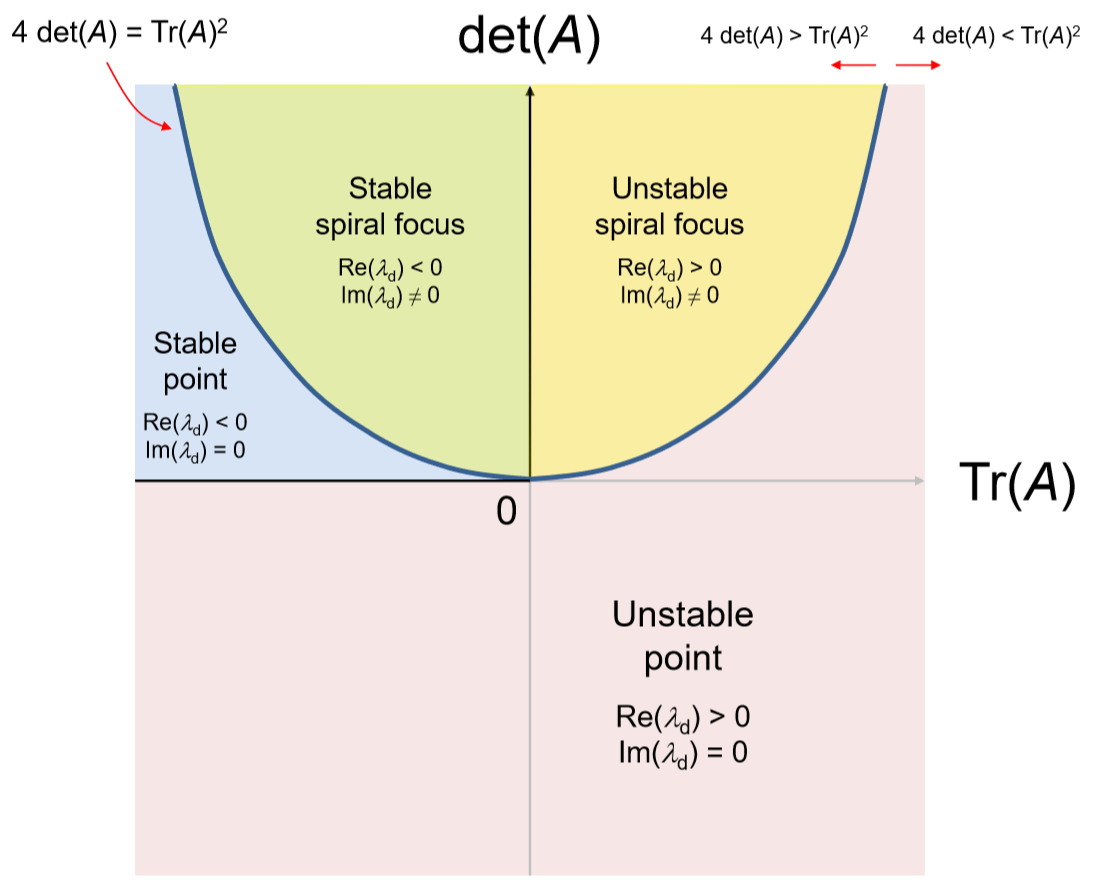
Show that the unstable points with \(det(A) < 0\) are saddle points.
Determine the stability of the following linear systems:
\[ \cdot \frac{dx}{dt}= \begin{pmatrix} -1 & 2\\2 &-2 \end{pmatrix} x \nonumber \]
\[\cdot \frac{dx}{dt} =\begin{pmatrix} 0.5 & -1.5\\ 1&-1\end{pmatrix} x \nonumber \]
Confirm the analytical result shown in Fig. 7.4.1 by conducting numerical simulations in Python and by drawing phase spaces of the system for several samples of \(A\).