9.2: Characteristics of Chaos

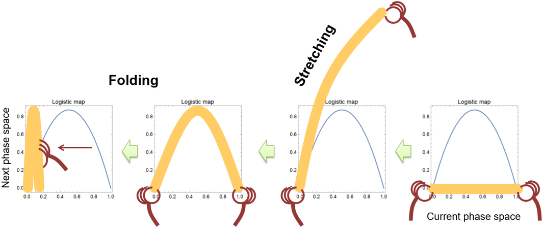
It is helpful to realize that there are two dynamical processes always going on in any kind of chaotic systems: stretching and folding [33]. Any chaotic system has a dynamical mechanism to stretch, and then fold, its phase space, like kneading pastry dough (Figure \(\PageIndex{1}\)). Imagine that you are keeping track of the location of a specific grain of flour in the dough while a pastry chef kneads the dough for a long period of time. Stretching the dough magnifies the tiny differences in position at microscopic scales to a larger, visible one, while folding the dough always keeps its extension within a finite, confined size. Note that folding is the primary source of nonlinearity that makes long-term predictions so hard—if the chef were simply stretching the dough all the time (which would look more like making ramen), you would still have a pretty good idea about where your favorite grain of flour would be after the stretching was completed. This stretching-and-folding view allows us to make another interpretation of chaos:

Stretching and Folding Phase Space

Chaos can be understood as a dynamical process in which microscopic information hidden in the details of a system’s state is dug out and expanded to a macroscopically visible scale (stretching), while the macroscopic information visible in the current system’s state is continuously discarded (folding).

Jul 24, 2018, 8:45 PM

http://beyondmicrofoundations.blogsp...2012-csss.html

https://elmer.unibas.ch/pendulum/lab.htm

Figure \(\PageIndex{1}\): Schematic illustration of strechting and folding taking place in a chaotic iterative map. The current phase space (right) is first stretched (middle right) and then folded (middle left and left) to generate the next phase spectra in each iteration.

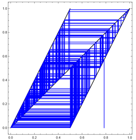
This kind of information flow-based explanation of chaos is quite helpful in understanding the essence of chaos from a multiscale perspective. This is particularly clear when you consider the saw map discussed in the previous exercise:

\[x_{t}= \text{fractional part of } 2x_{t-1} \label{9.1} \]

If you know binary notations of real numbers, it should be obvious that this iterative map is simply shifting the bit string in \(x\) always to the left, while forgetting the bits that came before the decimal point. And yet, such a simple arithmetic operation can still create chaos, if the initial condition is an irrational number (Figure \(\PageIndex{2}\))! This is because an irrational number contains an infinite length of digits and chaos continuously digs them out to produce a fluctuating behavior at a visible scale.

Figure \(\PageIndex{1}\): Cobweb plot for the saw map with \(\pi/4\) as the initial condition.

Exercise \(\PageIndex{1}\)

The saw map can also show chaos even from a rational initial condition, if its behavior is manually simulated by hand on a cobweb plot. Explain why.