9.3: Lyapunov Exponent
- Page ID
- 7819
\( \newcommand{\vecs}[1]{\overset { \scriptstyle \rightharpoonup} {\mathbf{#1}} } \)
\( \newcommand{\vecd}[1]{\overset{-\!-\!\rightharpoonup}{\vphantom{a}\smash {#1}}} \)
\( \newcommand{\id}{\mathrm{id}}\) \( \newcommand{\Span}{\mathrm{span}}\)
( \newcommand{\kernel}{\mathrm{null}\,}\) \( \newcommand{\range}{\mathrm{range}\,}\)
\( \newcommand{\RealPart}{\mathrm{Re}}\) \( \newcommand{\ImaginaryPart}{\mathrm{Im}}\)
\( \newcommand{\Argument}{\mathrm{Arg}}\) \( \newcommand{\norm}[1]{\| #1 \|}\)
\( \newcommand{\inner}[2]{\langle #1, #2 \rangle}\)
\( \newcommand{\Span}{\mathrm{span}}\)
\( \newcommand{\id}{\mathrm{id}}\)
\( \newcommand{\Span}{\mathrm{span}}\)
\( \newcommand{\kernel}{\mathrm{null}\,}\)
\( \newcommand{\range}{\mathrm{range}\,}\)
\( \newcommand{\RealPart}{\mathrm{Re}}\)
\( \newcommand{\ImaginaryPart}{\mathrm{Im}}\)
\( \newcommand{\Argument}{\mathrm{Arg}}\)
\( \newcommand{\norm}[1]{\| #1 \|}\)
\( \newcommand{\inner}[2]{\langle #1, #2 \rangle}\)
\( \newcommand{\Span}{\mathrm{span}}\) \( \newcommand{\AA}{\unicode[.8,0]{x212B}}\)
\( \newcommand{\vectorA}[1]{\vec{#1}} % arrow\)
\( \newcommand{\vectorAt}[1]{\vec{\text{#1}}} % arrow\)
\( \newcommand{\vectorB}[1]{\overset { \scriptstyle \rightharpoonup} {\mathbf{#1}} } \)
\( \newcommand{\vectorC}[1]{\textbf{#1}} \)
\( \newcommand{\vectorD}[1]{\overrightarrow{#1}} \)
\( \newcommand{\vectorDt}[1]{\overrightarrow{\text{#1}}} \)
\( \newcommand{\vectE}[1]{\overset{-\!-\!\rightharpoonup}{\vphantom{a}\smash{\mathbf {#1}}}} \)
\( \newcommand{\vecs}[1]{\overset { \scriptstyle \rightharpoonup} {\mathbf{#1}} } \)
\( \newcommand{\vecd}[1]{\overset{-\!-\!\rightharpoonup}{\vphantom{a}\smash {#1}}} \)
\(\newcommand{\avec}{\mathbf a}\) \(\newcommand{\bvec}{\mathbf b}\) \(\newcommand{\cvec}{\mathbf c}\) \(\newcommand{\dvec}{\mathbf d}\) \(\newcommand{\dtil}{\widetilde{\mathbf d}}\) \(\newcommand{\evec}{\mathbf e}\) \(\newcommand{\fvec}{\mathbf f}\) \(\newcommand{\nvec}{\mathbf n}\) \(\newcommand{\pvec}{\mathbf p}\) \(\newcommand{\qvec}{\mathbf q}\) \(\newcommand{\svec}{\mathbf s}\) \(\newcommand{\tvec}{\mathbf t}\) \(\newcommand{\uvec}{\mathbf u}\) \(\newcommand{\vvec}{\mathbf v}\) \(\newcommand{\wvec}{\mathbf w}\) \(\newcommand{\xvec}{\mathbf x}\) \(\newcommand{\yvec}{\mathbf y}\) \(\newcommand{\zvec}{\mathbf z}\) \(\newcommand{\rvec}{\mathbf r}\) \(\newcommand{\mvec}{\mathbf m}\) \(\newcommand{\zerovec}{\mathbf 0}\) \(\newcommand{\onevec}{\mathbf 1}\) \(\newcommand{\real}{\mathbb R}\) \(\newcommand{\twovec}[2]{\left[\begin{array}{r}#1 \\ #2 \end{array}\right]}\) \(\newcommand{\ctwovec}[2]{\left[\begin{array}{c}#1 \\ #2 \end{array}\right]}\) \(\newcommand{\threevec}[3]{\left[\begin{array}{r}#1 \\ #2 \\ #3 \end{array}\right]}\) \(\newcommand{\cthreevec}[3]{\left[\begin{array}{c}#1 \\ #2 \\ #3 \end{array}\right]}\) \(\newcommand{\fourvec}[4]{\left[\begin{array}{r}#1 \\ #2 \\ #3 \\ #4 \end{array}\right]}\) \(\newcommand{\cfourvec}[4]{\left[\begin{array}{c}#1 \\ #2 \\ #3 \\ #4 \end{array}\right]}\) \(\newcommand{\fivevec}[5]{\left[\begin{array}{r}#1 \\ #2 \\ #3 \\ #4 \\ #5 \\ \end{array}\right]}\) \(\newcommand{\cfivevec}[5]{\left[\begin{array}{c}#1 \\ #2 \\ #3 \\ #4 \\ #5 \\ \end{array}\right]}\) \(\newcommand{\mattwo}[4]{\left[\begin{array}{rr}#1 \amp #2 \\ #3 \amp #4 \\ \end{array}\right]}\) \(\newcommand{\laspan}[1]{\text{Span}\{#1\}}\) \(\newcommand{\bcal}{\cal B}\) \(\newcommand{\ccal}{\cal C}\) \(\newcommand{\scal}{\cal S}\) \(\newcommand{\wcal}{\cal W}\) \(\newcommand{\ecal}{\cal E}\) \(\newcommand{\coords}[2]{\left\{#1\right\}_{#2}}\) \(\newcommand{\gray}[1]{\color{gray}{#1}}\) \(\newcommand{\lgray}[1]{\color{lightgray}{#1}}\) \(\newcommand{\rank}{\operatorname{rank}}\) \(\newcommand{\row}{\text{Row}}\) \(\newcommand{\col}{\text{Col}}\) \(\renewcommand{\row}{\text{Row}}\) \(\newcommand{\nul}{\text{Nul}}\) \(\newcommand{\var}{\text{Var}}\) \(\newcommand{\corr}{\text{corr}}\) \(\newcommand{\len}[1]{\left|#1\right|}\) \(\newcommand{\bbar}{\overline{\bvec}}\) \(\newcommand{\bhat}{\widehat{\bvec}}\) \(\newcommand{\bperp}{\bvec^\perp}\) \(\newcommand{\xhat}{\widehat{\xvec}}\) \(\newcommand{\vhat}{\widehat{\vvec}}\) \(\newcommand{\uhat}{\widehat{\uvec}}\) \(\newcommand{\what}{\widehat{\wvec}}\) \(\newcommand{\Sighat}{\widehat{\Sigma}}\) \(\newcommand{\lt}{<}\) \(\newcommand{\gt}{>}\) \(\newcommand{\amp}{&}\) \(\definecolor{fillinmathshade}{gray}{0.9}\)Finally, I would like to introduce one useful analytical metric that can help characterize chaos. It is called the Lyapunov exponent, which measures how quickly an infinitesimally small distance between two initially close states grows over time:
\[F^{t}(x_0 + ε)−F^{t}(x_0) ≈ εe^{λt} \label{9.2} \]
The left hand side is the distance between two initially close states after \(t\) steps, and the right hand side is the assumption that the distance grows exponentially over time. The exponent \(λ\) measured for a long period of time (ideally \(t → ∞)\) is the Lyapunov exponent. If \(λ > 0\), small distances grow indefinitely over time, which means the stretching mechanism is in effect. Or if \(λ < 0\), small distances don’t grow indefinitely, i.e., the system settles down into a periodic trajectory eventually. Note that the Lyapunov exponent characterizes only stretching, but as we discussed before, stretching is not the only mechanism of chaos. You should keep in mind that the folding mechanism is not captured in this Lyapunov exponent.
We can do a little bit of mathematical derivation to transform Equation \ref{9.2} into a more easily computable form:
\[e^{λt} ≈ \frac{|F^{t}(x_{0} + ε)−F^{t}(x_{0})|}{ ε} \label{9.3} \]
\[\begin{align} λ &= \lim _{t→∞,ε→0} \frac{1} {t} \log{\frac{|F^{t}(x_{0} +\varepsilon)-F^{t}(x_{0})|}{\varepsilon}}\label{9.4} \\[4pt] &= \lim_{ t→∞ 1, ε→0}\frac{1} {t} \log {|\frac{dF} {dx}| _{x=x_0}|}\label{9.5} \end{align} \]
(applying the chain rule of differentiation...)
\[λ = \lim_{t→∞}\frac{ 1}{ t} \log {|\frac{dF}{ dx}}|_{ x=F^{t−1}(x_0)=x_{t−1}} · \frac{dF}{ dx}|_{ x=F^{t−2}(x_0)=x_{t−2}} ···· \frac{dF}{ dx}|_{x=x_{0}}\label{9.6} \]
\[ \lim_{t \rightarrow \infty }\frac{1}{t} \sum^{t-1}_{i=0} \log{|\frac{dF}{ dx}|_{ x=x_{i} }|} \label{9.7} \]
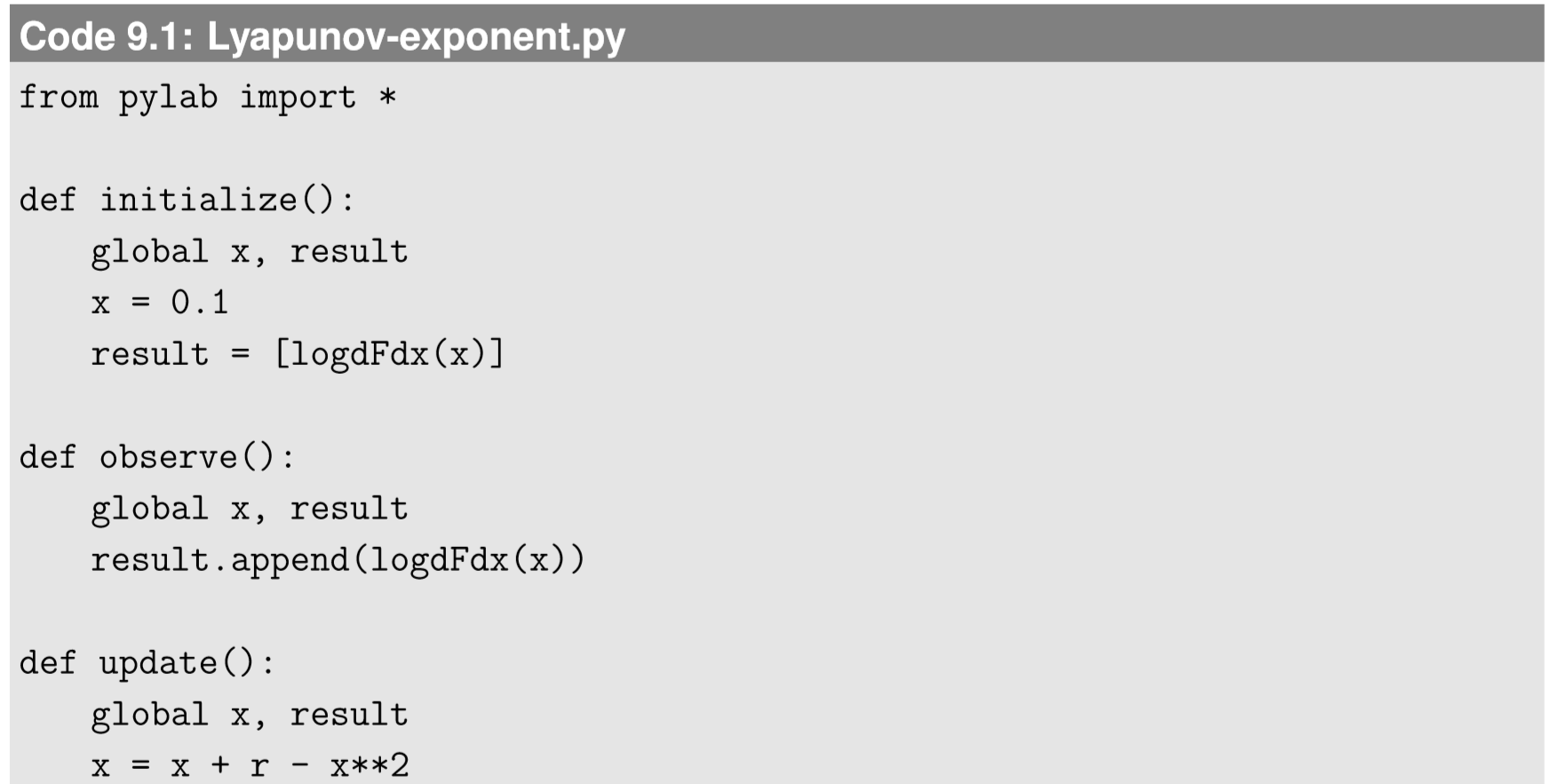
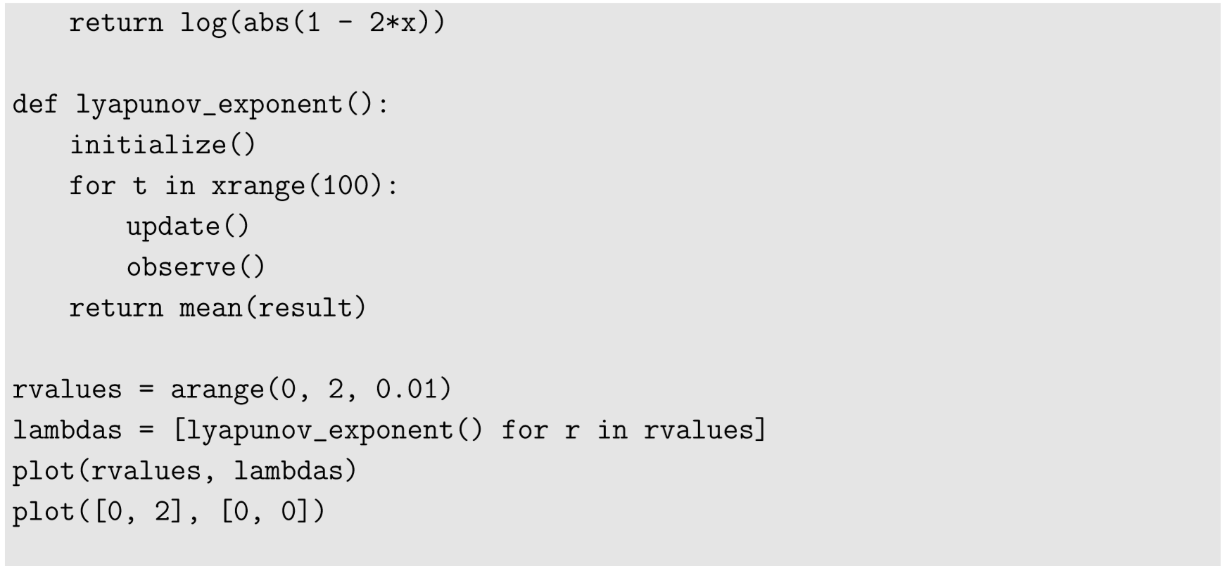
The final result is quite simple—the Lyapunov exponent is a time average of \(log|\frac{dF}{dx}|\) at every state the system visits over the course of the simulation. This is very easy to compute numerically. Here is an example of computing the Lyapunov exponent of Eq. 8.4.3 over varying \(r\):
Figure 9.3.1 shows the result. By comparing this figure with the bifurcation diagram (Fig. 8.4.3), you will notice that the parameter range where the Lyapunov exponent takes positive values nicely matches the range where the system shows chaotic behavior. Also, whenever a bifurcation occurs (e.g., \(r = 1\), \(1.5\), etc.), the Lyapunov exponent touches the \(λ = 0\) line, indicating the criticality of those parameter values. Finally, there are several locations in the plot where the Lyapunov exponent diverges to negative infinity (they may not look so, but they are indeed going infinitely deep). Such values occur when the system converges to an extremely stable equilibrium point with \(\frac{dF^{t}}{dx}_{|x=x_{0}} ≈ 0\) for certain \(t\). Since the definition of the Lyapunov exponent contains logarithms of this derivative, if it becomes zero, the exponent diverges to negative infinity as well.
Plot the Lyapunov exponent of the logistic map (Eq. (\ref{8.4.9})) for \(0 < r < 4\), and compare the result with its bifurcation diagram.
Plot the bifurcation diagram and the Lyapunov exponent of the following discrete-time dynamical system for \(r > 0\):
\[x_{t}= cos^{2}(rx_{t-1})\label{9.8} \]
Then explain in words how its dynamics change over \(r\).