1: IEEE Arithmetic

Last updated
Save as PDF

Page ID: 93661

$ \newcommand{\vecs}[1]{\overset { \scriptstyle \rightharpoonup} {\mathbf{#1}} } $ $ \newcommand{\vecd}[1]{\overset{-\!-\!\rightharpoonup}{\vphantom{a}\smash {#1}}} $$\newcommand{\id}{\mathrm{id}}$ $ \newcommand{\Span}{\mathrm{span}}$ $ \newcommand{\kernel}{\mathrm{null}\,}$ $ \newcommand{\range}{\mathrm{range}\,}$ $ \newcommand{\RealPart}{\mathrm{Re}}$ $ \newcommand{\ImaginaryPart}{\mathrm{Im}}$ $ \newcommand{\Argument}{\mathrm{Arg}}$ $ \newcommand{\norm}[1]{\| #1 \|}$ $ \newcommand{\inner}[2]{\langle #1, #2 \rangle}$ $ \newcommand{\Span}{\mathrm{span}}$ $\newcommand{\id}{\mathrm{id}}$ $ \newcommand{\Span}{\mathrm{span}}$ $ \newcommand{\kernel}{\mathrm{null}\,}$ $ \newcommand{\range}{\mathrm{range}\,}$ $ \newcommand{\RealPart}{\mathrm{Re}}$ $ \newcommand{\ImaginaryPart}{\mathrm{Im}}$ $ \newcommand{\Argument}{\mathrm{Arg}}$ $ \newcommand{\norm}[1]{\| #1 \|}$ $ \newcommand{\inner}[2]{\langle #1, #2 \rangle}$ $ \newcommand{\Span}{\mathrm{span}}$$\newcommand{\AA}{\unicode[.8,0]{x212B}}$

Definitions

The real line is continuous, while computer numbers are discrete. We learn here how numbers are represented in the computer, and how this can lead to round-off errors. A number can be represented in the computer as a signed or unsigned integer, or as a real (floating point) number. We introduce the following definitions:

$\begin{array}{lll}\text { Bit } & =0 \text { or } 1 & \\ \text { Byte } & =8 \text { bits } & \\ \text { Word } & =\text { Reals: } & 4 \text { bytes (single precision) } \\ & & 8 \text { bytes (double precision) } \\ & =\text { Integers: } & 1,2,4, \text { or } 8 \text { byte signed } \\ & & 1,2,4, \text { or } 8 \text { byte unsigned }\end{array}$

Typically, scientific computing in MATLAB is in double precision using 8-byte real numbers. Single precision may be used infrequently in large problems to conserve memory. Integers may also be used infrequently in special situations. Since double precision is the default-and what will be used in this class-we will focus here on its representation.

IEEE double precision format

Double precision makes use of 8 byte words ( 64 bits), and usually results in sufficiently accurate computations. The format for a double precision number is

$clipboard_eb44de7f1525b19f28db470274f436150.png$

\[ \nonumber \#=(-1)^s \times 2^{e-1023} \times 1.f, \nonumber \]

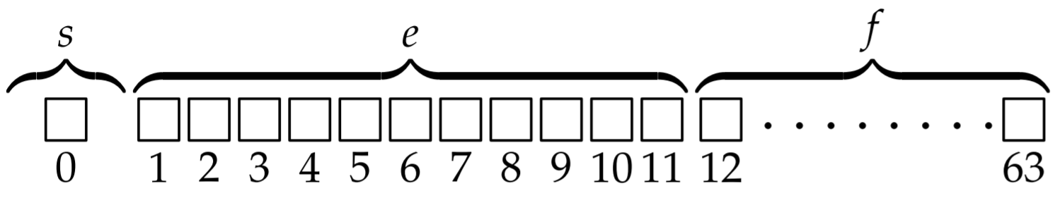
where $\mathrm{s}$ is the sign bit, e is the biased exponent, and 1.f (using a binary point) is the significand. We see that the 64 bits are distributed so that the sign uses 1-bit, the exponent uses 11-bits, and the significand uses 52-bits. The distribution of bits between the exponent and the significand is to reconcile two conflicting desires: that the numbers should range from very large to very small values, and that the relative spacing between numbers should be small.

Machine numbers

We show for illustration how the numbers 1,2 , and $1 / 2$ are represented in double precision. For the number 1 , we write

\[1.0=(-1)^{0} \times 2^{(1023-1023)} \times 1.0 . \nonumber \]

From (1.1), we find $\mathrm{s}=0, \mathrm{e}=1023$, and $\mathrm{f}=0$. Now

\[1023=01111111111 \text { (base 2), } \nonumber \]

so that the machine representation of the number 1 is given by

\[0011111111110000 \ldots 0000 \text {. } \nonumber \]

One can view the machine representation of numbers in MATLAB using the format hex command. MATLAB then displays the hex number corresponding to the binary machine number. Hex maps four bit binary numbers to a single character, where the binary numbers corresponding to the decimal 0-9 are mapped to the same decimal numbers, and the binary numbers corresponding to $10-15$ are mapped to a-f. The hex representation of the number 1 given by (1.3) is therefore given by

\[3 f f 0\, 0000\, 0000\, 0000 \text {. } \nonumber \]

For the number 2, we have

\[2.0=(-1)^{0} \times 2^{(1024-1023)} \times 1.0, \nonumber \]

with binary representation

\[0100\, 0000\, 0000\, 0000 \ldots 0000 \nonumber \]

and hex representation

\[4000\, 0000\, 0000\, 0000 . \nonumber \]

For the number $1 / 2$, we have

\[2.0=(-1)^{0} \times 2^{(1022-1023)} \times 1.0, \nonumber \]

with binary representation

\[0011\, 1111\, 1110\, 0000 \ldots 0000 \nonumber \]

and hex representation

\[4 \mathrm{fe} 0\, 0000\, 0000\, 0000 . \nonumber \]

The numbers 1,2 and $1 / 2$ can be represented exactly in double precision. But very large integers, and most real numbers can not. For example, the number $1 / 3$ is inexact, and so is $1 / 5$, which we consider here. We write

\[\begin{aligned} \frac{1}{5} &=(-1)^{0} \times \frac{1}{8} \times\left(1+\frac{3}{5}\right) \\ &=(-1)^{0} \times 2^{1020-1023} \times\left(1+\frac{3}{5}\right) \end{aligned} \nonumber \]

so that $\mathrm{s}=0, \mathrm{e}=1020=01111111100$ (base 2), and $\mathrm{f}=3 / 5$. The reason 1/5 is inexact is that $3 / 5$ does not have a finite representation in binary. To convert $3 / 5$ to binary, we multiply successively by 2 as follows:

\[ \begin{array}{lll} 0.6 \ldots & \qquad \qquad \qquad & 0. \\ 1.2 \ldots & \qquad \qquad \qquad & 0.1 \\ 0.4 \ldots & \qquad \qquad \qquad & 0.10 \\ 0.8 \ldots & \qquad \qquad \qquad & 0.100 \\ 1.6 \ldots & \qquad \qquad \qquad & 0.1001 \\ \qquad \text{etc} & & \end{array} \nonumber \]

so that $3 / 5$ exactly in binary is $0 . \overline{1001}$, where the bar denotes an endless repetition. With only 52 bits to represent $\mathrm{f}$, the fraction $3 / 5$ is inexact and we have

\[\mathrm{f}=10011001 \ldots 10011010 \text {, } \nonumber \]

where we have rounded the repetitive end of the number $\overline{1001}$ to the nearest binary number 1010. Here the rounding is up because the 53-bit is a 1 followed by not all zeros. But rounding can also be down if the 53 bit is a 0 . Exactly on the boundary (the 53-bit is a 1 followed by all zeros), rounding is to the nearest even number. In this special situation that occurs only rarely, if the 52-bit is a 0 , then rounding is down, and if the 52 bit is a 1 , then rounding is up.

The machine number $1 / 5$ is therefore represented as

\[00111111110010011001 \ldots 10011010 \text {, } \nonumber \]

or in hex,

3fc999999999999a

The small error in representing a number such as $1 / 5$ in double precision usually makes little difference in a computation. One is usually satisfied to obtain results accurate to a few significant digits. Nevertheless, computational scientists need to be aware that most numbers are not represented exactly.

For example, consider subtracting what should be two identical real numbers that are not identical in the computer. In MATLAB, if one enters on the command line

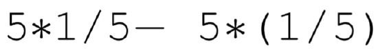
$clipboard_e6345f788992c11fcbb05ad74d37dacb0.png$

the resulting answer is 0 , as one would expect. But if one enters

$clipboard_e1affab3b6c3837e19c2c41f8a38dd696.png$

the resulting answer is $-2.2204 \mathrm{e}-16$, a number slightly different than zero. The reason for this error is that although the number $5^{2} * 1 / 5^{2}=25 / 25=1$ can be represented exactly, the number $5^{2} *(1 / 5)^{2}$ is inexact and slightly greater than one. Testing for exactly zero in a calculation that depends on the cancelation of real numbers, then, may not work. More problematic, though, are calculations that subtract two large numbers with the hope of obtaining a sensible small number. A total loss of precision of the small number may occur.

Special numbers

Both the largest and smallest exponent are reserved in IEEE arithmetic. When $\mathrm{f}=0$, the largest exponent, $\mathrm{e}=11111111111$, is used to represent $\pm \infty$ (written in MATLAB as Inf and - Inf). When $\mathrm{f} \neq 0$, the largest exponent is used to represent ’not a number’ (written in MATLAB as NaN). IEEE arithmetic also implements what is called denormal numbers, also called graceful underflow. It reserves the smallest exponent, $\mathrm{e}=00000000000$, to represent numbers for which the representation changes from 1.f to $0 . f$.

With the largest exponent reserved, the largest positive double precision number has $\mathrm{s}=0, \mathrm{e}=11111111110=2046$, and $\mathrm{f}=11111111 \ldots 1111=1-2^{-52} .$ Called realmax in MATLAB, we have

$clipboard_e883aa55ae077b24adf9ef753a5c684bd.png$

With the smallest exponent reserved, the smallest positive double precision number has $\mathrm{s}=0, \mathrm{e}=00000000001=1$, and $\mathrm{f}=00000000 \ldots 0000=0$. Called realmin in MATLAB, we have

$clipboard_e1d2adbd9ee68735fa214dc202590392a.png$

Above realmax, one obtains Inf, and below realmin, one obtains first denormal numbers and then 0 .

Another important number is called machine epsilon (called eps in MATLAB). Machine epsilon is defined as the distance between 1 and the next largest number. If $0 \leq \delta<e p s / 2$, then $1+\delta=1$ in computer math. Also since

\[x+y=x(1+y / x), \nonumber \]

if $0 \leq y / x<e p s / 2$, then $x+y=x$ in computer math.

Now, the number 1 in double precision IEEE format is written as

\[1=2^{0} \times 1.000 \ldots 0, \nonumber \]

with 520 ’s following the binary point. The number just larger than 1 has a 1 in the 52nd position after the decimal point. Therefore,

\[\text { eps }=2^{-52} \approx 2.2204 e-016 \text {. } \nonumber \]

What is the distance between 1 and the number just smaller than 1 ? Here, the number just smaller than one can be written as

\[2^{-1} \times 1.111 \ldots 1=2^{-1}\left(1+\left(1-2^{-52}\right)\right)=1-2^{-53} \nonumber \]

Therefore, this distance is $2^{-53}=\mathrm{eps} / 2$.

Here, we observe that the spacing between numbers is uniform between powers of 2, but changes by a factor of two with each additional power of two. For example, the spacing of numbers between 1 and 2 is $2^{-52}$, between 2 and 4 is $2^{-51}$, between 4 and 8 is $2^{-50}$, etc. An exception occurs for denormal numbers, where the spacing becomes uniform all the way down to zero. Denormal numbers implement a graceful underflow, and are not to be used for normal computation.

Roundoff error

Consider solving the quadratic equation

\[x^{2}+2 b x-1=0, \nonumber \]

where $b$ is a parameter. The quadratic formula yields the two solutions

\[x_{\pm}=-b \pm \sqrt{b^{2}+1} . \nonumber \]

Now, consider the solution with $b>0$ and $x>0$ (the $x_{+}$solution) given by

\[x=-b+\sqrt{b^{2}+1} . \nonumber \]

As $b \rightarrow \infty$

\[\begin{aligned} x &=-b+\sqrt{b^{2}+1} \\ &=-b+b \sqrt{1+1 / b^{2}} \\ &=b\left(\sqrt{1+1 / b^{2}}-1\right) \\ & \approx b\left(1+\frac{1}{2 b^{2}}-1\right) \\ &=\frac{1}{2 b} . \end{aligned} \nonumber \]

Now in double precision, realmin $\approx 2.2 \times 10^{-308}$ and in professional software one would like $x$ to be accurate to this value before it goes to 0 via denormal numbers. Therefore, $x$ should be computed accurately to $b \approx 1 /(2 \times$ realmin $) \approx 2 \times 10^{307}$. What happens if we compute (1.19) directly? Then $x=0$ when $b^{2}+1=b^{2}$, or $1+1 / b^{2}=1$. Therefore, $x=0$ when $1 / b^{2}<$ eps $/ 2$, or $b>\sqrt{2 / e p s} \approx 10^{8}$.

The way that a professional mathematical software designer solves this problem is to compute the solution for $x$ when $b>0$ as

\[x=\frac{1}{b+\sqrt{b^{2}+1}} . \nonumber \]

In this form, when $b^{2}+1=b^{2}$, then $x=1 / 2 b$, which is the correct asymptotic form.