5: Linear Algebra

Consider the system of \(n\) linear equations and \(n\) unknowns, given by

\[\begin{array}{cc} a_{11} x_{1}+a_{12} x_{2}+\cdots+a_{1 n} x_{n}= & b_{1}, \\ a_{21} x_{1}+a_{22} x_{2}+\cdots+a_{2 n} x_{n}= & b_{2}, \\ \vdots & \vdots \\ a_{n 1} x_{1}+a_{n 2} x_{2}+\cdots+a_{n n} x_{n}= & b_{n} . \end{array} \nonumber \]

We can write this system as the matrix equation

\[A x=b \text {, } \nonumber \]

with

\[\mathrm{A}=\left(\begin{array}{cccc} a_{11} & a_{12} & \cdots & a_{1 n} \\ a_{21} & a_{22} & \cdots & a_{2 n} \\ \vdots & \vdots & \ddots & \vdots \\ a_{n 1} & a_{n 2} & \cdots & a_{n n} \end{array}\right), \quad \mathbf{x}=\left(\begin{array}{c} x_{1} \\ x_{2} \\ \vdots \\ x_{n} \end{array}\right), \quad \mathbf{b}=\left(\begin{array}{c} b_{1} \\ b_{2} \\ \vdots \\ b_{n} \end{array}\right) \nonumber \]

This chapter details the numerical solution of (5.1).

Gaussian Elimination

The standard numerical algorithm to solve a system of linear equations is called Gaussian Elimination. We can illustrate this algorithm by example.

Consider the system of equations

\[\begin{aligned} -3 x_{1}+2 x_{2}-x_{3} &=-1, \\ 6 x_{1}-6 x_{2}+7 x_{3} &=-7, \\ 3 x_{1}-4 x_{2}+4 x_{3} &=-6 . \end{aligned} \nonumber \]

To perform Gaussian elimination, we form an Augmented Matrix by combining the matrix A with the column vector \(\vec{b}\) :

\[\left(\begin{array}{rrrr} -3 & 2 & -1 & -1 \\ 6 & -6 & 7 & -7 \\ 3 & -4 & 4 & -6 \end{array}\right) \text {. } \nonumber \]

Row reduction is then performed on this matrix. Allowed operations are (1) multiply any row by a constant, (2) add multiple of one row to another row, (3) interchange the order of any rows. The goal is to convert the original matrix into an upper-triangular matrix. We start with the first row of the matrix and work our way down as follows. First we multiply the first row by 2 and add it to the second row, and add the first row to the third row:

\[\left(\begin{array}{rrrr} -3 & 2 & -1 & -1 \\ 0 & -2 & 5 & -9 \\ 0 & -2 & 3 & -7 \end{array}\right) \text {. } \nonumber \]

We then go to the second row. We multiply this row by \(-1\) and add it to the third row:

\[\left(\begin{array}{rrrr} -3 & 2 & -1 & -1 \\ 0 & -2 & 5 & -9 \\ 0 & 0 & -2 & 2 \end{array}\right) \text {. } \nonumber \]

The resulting equations can be determined from the matrix and are given by

\[\begin{aligned} -3 x_{1}+2 x_{2}-x_{3} &=-1 \\ -2 x_{2}+5 x_{3} &=-9 \\ -2 x_{3} &=2 . \end{aligned} \nonumber \]

These equations can be solved by backward substitution, starting from the last equation and working backwards. We have

\[\begin{aligned} &-2 x_{3}=2 \rightarrow x_{3}=-1 \\ &-2 x_{2}=-9-5 x_{3}=-4 \rightarrow x_{2}=2 \\ &-3 x_{1}=-1-2 x_{2}+x_{3}=-6 \rightarrow x_{1}=2 \end{aligned} \nonumber \]

Therefore,

\[\left(\begin{array}{l} x_{1} \\ x_{2} \\ x_{3} \end{array}\right)=\left(\begin{array}{r} 2 \\ 2 \\ -1 \end{array}\right) \nonumber \]

LU decomposition

The process of Gaussian Elimination also results in the factoring of the matrix A to

\[\mathrm{A}=\mathrm{LU} \text {, } \nonumber \]

where \(\mathrm{L}\) is a lower triangular matrix and \(\mathrm{U}\) is an upper triangular matrix. Using the same matrix A as in the last section, we show how this factorization is realized. We have

\[\left(\begin{array}{rrr} -3 & 2 & -1 \\ 6 & -6 & 7 \\ 3 & -4 & 4 \end{array}\right) \rightarrow\left(\begin{array}{rrr} -3 & 2 & -1 \\ 0 & -2 & 5 \\ 0 & -2 & 3 \end{array}\right)=\mathrm{M}_{1} \mathrm{~A} \nonumber \]

where

\[\mathrm{M}_{1} \mathrm{~A}=\left(\begin{array}{lll} 1 & 0 & 0 \\ 2 & 1 & 0 \\ 1 & 0 & 1 \end{array}\right)\left(\begin{array}{rrr} -3 & 2 & -1 \\ 6 & -6 & 7 \\ 3 & -4 & 4 \end{array}\right)=\left(\begin{array}{rrr} -3 & 2 & -1 \\ 0 & -2 & 5 \\ 0 & -2 & 3 \end{array}\right) . \nonumber \]

Note that the matrix \(\mathrm{M}_{1}\) performs row elimination on the first column. Two times the first row is added to the second row and one times the first row is added to the third row. The entries of the column of \(\mathrm{M}_{1}\) come from \(2=-(6 /-3)\) and \(1=-(3 /-3)\) as required for row elimination. The number \(-3\) is called the pivot.

The next step is

\[\left(\begin{array}{rrr} -3 & 2 & -1 \\ 0 & -2 & 5 \\ 0 & -2 & 3 \end{array}\right) \rightarrow\left(\begin{array}{rrr} -3 & 2 & -1 \\ 0 & -2 & 5 \\ 0 & 0 & -2 \end{array}\right)=\mathrm{M}_{2}\left(\mathrm{M}_{1} \mathrm{~A}\right) \text {, } \nonumber \]

where

\[\mathrm{M}_{2}\left(\mathrm{M}_{1} \mathrm{~A}\right)=\left(\begin{array}{rrr} 1 & 0 & 0 \\ 0 & 1 & 0 \\ 0 & -1 & 1 \end{array}\right)\left(\begin{array}{rrr} -3 & 2 & -1 \\ 0 & -2 & 5 \\ 0 & -2 & 3 \end{array}\right)=\left(\begin{array}{rrr} -3 & 2 & -1 \\ 0 & -2 & 5 \\ 0 & 0 & -2 \end{array}\right) . \nonumber \]

Here, \(\mathrm{M}_{2}\) multiplies the second row by \(-1=-(-2 /-2)\) and adds it to the third row. The pivot is \(-2\).

We now have

\[\mathrm{M}_{2} \mathrm{M}_{1} \mathrm{~A}=\mathrm{U} \nonumber \]

or

\[\mathrm{A}=\mathrm{M}_{1}^{-1} \mathrm{M}_{2}^{-1} \mathrm{U} \text {. } \nonumber \]

The inverse matrices are easy to find. The matrix \(\mathrm{M}_{1}\) multiples the first row by 2 and adds it to the second row, and multiplies the first row by 1 and adds it to the third row. To invert these operations, we need to multiply the first row by \(-2\) and add it to the second row, and multiply the first row by \(-1\) and add it to the third row. To check, with

\[\mathrm{M}_{1} \mathrm{M}_{1}^{-1}=\mathrm{I}, \nonumber \]

we have

\[\left(\begin{array}{lll} 1 & 0 & 0 \\ 2 & 1 & 0 \\ 1 & 0 & 1 \end{array}\right)\left(\begin{array}{rrr} 1 & 0 & 0 \\ -2 & 1 & 0 \\ -1 & 0 & 1 \end{array}\right)=\left(\begin{array}{lll} 1 & 0 & 0 \\ 0 & 1 & 0 \\ 0 & 0 & 1 \end{array}\right) \text {. } \nonumber \]

Similarly,

\[\mathrm{M}_{2}^{-1}=\left(\begin{array}{ccc} 1 & 0 & 0 \\ 0 & 1 & 0 \\ 0 & 1 & 1 \end{array}\right) \nonumber \]

Therefore,

\[\mathrm{L}=\mathrm{M}_{1}^{-1} \mathrm{M}_{2}^{-1} \nonumber \]

is given by

\[\mathrm{L}=\left(\begin{array}{rll} 1 & 0 & 0 \\ -2 & 1 & 0 \\ -1 & 0 & 1 \end{array}\right)\left(\begin{array}{lll} 1 & 0 & 0 \\ 0 & 1 & 0 \\ 0 & 1 & 1 \end{array}\right)=\left(\begin{array}{rrr} 1 & 0 & 0 \\ -2 & 1 & 0 \\ -1 & 1 & 1 \end{array}\right) \nonumber \]

which is lower triangular. The off-diagonal elements of \(\mathrm{M}_{1}^{-1}\) and \(\mathrm{M}_{2}^{-1}\) are simply combined to form L. Our LU decomposition is therefore

\[\left(\begin{array}{rrr} -3 & 2 & -1 \\ 6 & -6 & 7 \\ 3 & -4 & 4 \end{array}\right)=\left(\begin{array}{rrr} 1 & 0 & 0 \\ -2 & 1 & 0 \\ -1 & 1 & 1 \end{array}\right)\left(\begin{array}{rrr} -3 & 2 & -1 \\ 0 & -2 & 5 \\ 0 & 0 & -2 \end{array}\right) \text {. } \nonumber \]

CHAPTER 5. LINEAR ALGEBRA Another nice feature of the LU decomposition is that it can be done by overwriting A, therefore saving memory if the matrix \(\mathrm{A}\) is very large.

The LU decomposition is useful when one needs to solve \(\mathrm{A} \mathbf{x}=\mathbf{b}\) for \(\mathbf{x}\) when \(\mathrm{A}\) is fixed and there are many different \(\mathbf{b}\) ’s. First one determines \(\mathrm{L}\) and \(\mathrm{U}\) using Gaussian elimination. Then one writes

\[(\mathrm{LU}) \mathbf{x}=\mathrm{L}(\mathrm{Ux})=\mathbf{b} \text {. } \nonumber \]

We let

\[\mathbf{y}=\mathrm{Ux}, \nonumber \]

and first solve

\[\text { Ly }=b \nonumber \]

for \(\mathbf{y}\) by forward substitution. We then solve

\[\mathrm{Ux}=\mathrm{y} \nonumber \]

for \(\mathbf{x}\) by backward substitution. If we count operations, we can show that solving (LU) \(\mathbf{x}=\mathbf{b}\) is substantially faster once \(\mathrm{L}\) and \(\mathrm{U}\) are in hand than solving \(\mathrm{Ax}=\mathbf{b}\) directly by Gaussian elimination.

We now illustrate the solution of \(L U x=b\) using our previous example, where

\[\mathrm{L}=\left(\begin{array}{rrr} 1 & 0 & 0 \\ -2 & 1 & 0 \\ -1 & 1 & 1 \end{array}\right), \quad \mathrm{U}=\left(\begin{array}{rrr} -3 & 2 & -1 \\ 0 & -2 & 5 \\ 0 & 0 & -2 \end{array}\right), \quad \mathbf{b}=\left(\begin{array}{l} -1 \\ -7 \\ -6 \end{array}\right) \nonumber \]

With \(\mathbf{y}=\mathrm{Ux}\), we first solve \(\mathbf{L y}=\mathbf{b}\), that is

\[\left(\begin{array}{rrr} 1 & 0 & 0 \\ -2 & 1 & 0 \\ -1 & 1 & 1 \end{array}\right)\left(\begin{array}{l} y_{1} \\ y_{2} \\ y_{3} \end{array}\right)=\left(\begin{array}{l} -1 \\ -7 \\ -6 \end{array}\right) \text {. } \nonumber \]

Using forward substitution

\[\begin{aligned} &y_{1}=-1, \\ &y_{2}=-7+2 y_{1}=-9, \\ &y_{3}=-6+y_{1}-y_{2}=2 . \end{aligned} \nonumber \]

We now solve \(U x=\mathbf{y}\), that is

\[\left(\begin{array}{rrr} -3 & 2 & -1 \\ 0 & -2 & 5 \\ 0 & 0 & -2 \end{array}\right)\left(\begin{array}{l} x_{1} \\ x_{2} \\ x_{3} \end{array}\right)=\left(\begin{array}{r} -1 \\ -9 \\ 2 \end{array}\right) \text {. } \nonumber \]

Using backward substitution,

\[\begin{aligned} -2 x_{3} &=2 \rightarrow x_{3}=-1, \\ -2 x_{2} &=-9-5 x_{3}=-4 \rightarrow x_{2}=2, \\ -3 x_{1} &=-1-2 x_{2}+x_{3}=-6 \rightarrow x_{1}=2, \end{aligned} \nonumber \]

and we have once again determined

\[\left(\begin{array}{l} x_{1} \\ x_{2} \\ x_{3} \end{array}\right)=\left(\begin{array}{r} 2 \\ 2 \\ -1 \end{array}\right) \text {. } \nonumber \]

Partial pivoting

When performing Gaussian elimination, the diagonal element that one uses during the elimination procedure is called the pivot. To obtain the correct multiple, one uses the pivot as the divisor to the elements below the pivot. Gaussian elimination in this form will fail if the pivot is zero. In this situation, a row interchange must be performed.

Even if the pivot is not identically zero, a small value can result in big round-off errors. For very large matrices, one can easily lose all accuracy in the solution. To avoid these round-off errors arising from small pivots, row interchanges are made, and this technique is called partial pivoting (partial pivoting is in contrast to complete pivoting, where both rows and columns are interchanged). We will illustrate by example the LU decomposition using partial pivoting.

Consider

\[\mathrm{A}=\left(\begin{array}{rrr} -2 & 2 & -1 \\ 6 & -6 & 7 \\ 3 & -8 & 4 \end{array}\right) \text {. } \nonumber \]

We interchange rows to place the largest element (in absolute value) in the pivot, or \(a_{11}\), position. That is,

\[\mathrm{A} \rightarrow\left(\begin{array}{rrr} 6 & -6 & 7 \\ -2 & 2 & -1 \\ 3 & -8 & 4 \end{array}\right)=\mathrm{P}_{12} \mathrm{~A} \nonumber \]

where

\[\mathrm{P}_{12}=\left(\begin{array}{ccc} 0 & 1 & 0 \\ 1 & 0 & 0 \\ 0 & 0 & 1 \end{array}\right) \nonumber \]

is a permutation matrix that when multiplied on the left interchanges the first and second rows of a matrix. Note that \(P_{12}^{-1}=P_{12}\). The elimination step is then

\[\mathrm{P}_{12} \mathrm{~A} \rightarrow\left(\begin{array}{rrc} 6 & -6 & 7 \\ 0 & 0 & 4 / 3 \\ 0 & -5 & 1 / 2 \end{array}\right)=\mathrm{M}_{1} \mathrm{P}_{12} \mathrm{~A} \nonumber \]

where

\[\mathrm{M}_{1}=\left(\begin{array}{ccc} 1 & 0 & 0 \\ 1 / 3 & 1 & 0 \\ -1 / 2 & 0 & 1 \end{array}\right) . \nonumber \]

The final step requires one more row interchange:

\[\mathrm{M}_{1} \mathrm{P}_{12} \mathrm{~A} \rightarrow\left(\begin{array}{rrc} 6 & -6 & 7 \\ 0 & -5 & 1 / 2 \\ 0 & 0 & 4 / 3 \end{array}\right)=\mathrm{P}_{23} \mathrm{M}_{1} \mathrm{P}_{12} \mathrm{~A}=\mathrm{U} . \nonumber \]

Since the permutation matrices given by \(\mathrm{P}\) are their own inverses, we can write our result as

\[\left(\mathrm{P}_{23} \mathrm{M}_{1} \mathrm{P}_{23}\right) \mathrm{P}_{23} \mathrm{P}_{12} \mathrm{~A}=\mathrm{U} \text {. } \nonumber \]

Multiplication of \(\mathrm{M}\) on the left by \(\mathrm{P}\) interchanges rows while multiplication on the right by \(P\) interchanges columns. That is,

\[P_{23}\left(\begin{array}{ccc} 1 & 0 & 0 \\ 1 / 3 & 1 & 0 \\ -1 / 2 & 0 & 1 \end{array}\right) P_{23}=\left(\begin{array}{ccc} 1 & 0 & 0 \\ -1 / 2 & 0 & 1 \\ 1 / 3 & 1 & 0 \end{array}\right) P_{23}=\left(\begin{array}{ccc} 1 & 0 & 0 \\ -1 / 2 & 1 & 0 \\ 1 / 3 & 0 & 1 \end{array}\right) \text {. } \nonumber \]

The net result on \(\mathrm{M}_{1}\) is an interchange of the nondiagonal elements \(1 / 3\) and \(-1 / 2\).

We can then multiply by the inverse of \(\left(\mathrm{P}_{23} \mathrm{M}_{1} \mathrm{P}_{23}\right)\) to obtain

\[\mathrm{P}_{23} \mathrm{P}_{12} \mathrm{~A}=\left(\mathrm{P}_{23} \mathrm{M}_{1} \mathrm{P}_{23}\right)^{-1} \mathrm{U}, \nonumber \]

which we write as

\[\text { PA }=\text { LU. } \nonumber \]

Instead of L, MATLAB will write this as

\[\mathrm{A}=\left(\mathrm{P}^{-1} \mathrm{~L}\right) \mathrm{U} . \nonumber \]

For convenience, we will just denote \(\left(\mathrm{P}^{-1} \mathrm{~L}\right)\) by \(\mathrm{L}\), but by \(\mathrm{L}\) here we mean a permutated lower triangular matrix.

MATLAB programming

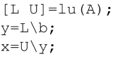
In MATLAB, to solve \(A \mathbf{x}=\mathbf{b}\) for \(\mathbf{x}\) using Gaussian elimination, one types

where \(\backslash\) solves for \(x\) using the most efficient algorithm available, depending on the form of A. If A is a general \(n \times n\) matrix, then first the LU decomposition of A is found using partial pivoting, and then \(x\) is determined from permuted forward and backward substitution. If \(\mathrm{A}\) is upper or lower triangular, then forward or backward substitution (or their permuted version) is used directly.

If there are many different right-hand-sides, one would first directly find the LU decomposition of A using a function call, and then solve using \(\backslash\). That is, one would iterate for different \(\mathbf{b}\) ’s the following expressions:

where the second and third lines can be shortened to

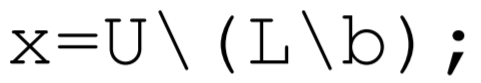
where the parenthesis are required. In lecture, I will demonstrate these solutions in MATLAB using the matrix \(A=[-3,2,-1 ; 6,-6,7 ; 3,-4,4]\) and the right-hand-side \(b=[-1 ;-7 ;-6]\), which is the example that we did by hand. Although we do not detail the algorithm here, MATLAB can also solve the linear algebra eigenvalue problem. Here, the mathematical problem to solve is given by

\[\mathrm{A} \mathbf{x}=\lambda \mathbf{x}, \nonumber \]

where \(\mathrm{A}\) is a square matrix, \(\lambda\) are the eigenvalues, and the associated \(\mathrm{x}^{\prime}\) s are the eigenvectors. The MATLAB subroutine that solves this problem is eig.m. To only find the eigenvalues of \(A\), one types

To find both the eigenvalues and eigenvectors, one types

More information can be found from the MATLAB help pages. One of the nice features about programming in MATLAB is that no great sin is commited if one uses a builtin function without spending the time required to fully understand the underlying algorithm.