5.1: Windows of periodicity scaling, the "linear" approximation

Windows of periodicity scaling

Windows of periodicity

Figure \(\PageIndex{1}\)

It is a commonly observed feature of chaotic dynamical systems [1] that, as a system parameter is varied, a stable period-n orbit appears (by a tangent bifurcation) which then undergoes a period-doubling cascade to chaos and finally terminates via a crisis. This parameter range between the tangent bifurcation and the final crisis is called a period-n window. Note, that the central part of the picture to the left is similar to the whole bifurcation diagram (see also at the bottom of the page).

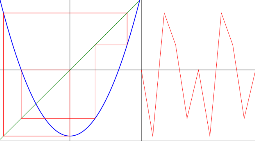
For c = -1.75 in the period-3 window stable and unstable period-3 orbits appear by a tangent bifurcation. The stable period-3 orbit is shown to the left below. If N = 3 is set (see to the right), we get 8 intersections (fixed points of f_c^o3) which correspond to two unstable fixed points and 6 points of the stable and unstable period-3 orbits of f_c .

Figure \(\PageIndex{2}\)

On the left picture the stable period-3 orbit goes through two "linear" and one central quadratic regions of the blue parabola. Therefore in the vicinity of x = 0 the map f_c^o3 is "quadratic-like" and iterations of the map repeat bifurcations of the original quadratic map f_c . This sheds light on the discussed similarity of windows of periodicity.

f_c^on map renormalization. The "linear" approximation

Consider a period-n window. Under iterations the critical orbit consecutively cycles through n narrow intervals S₁ → S₂ → S₃ → ... → S₁ each of width s_j (we choose S₁ to include the critical point x = 0).

Figure \(\PageIndex{3}\)

Figure \(\PageIndex{4}\)

 

Following we expand f_c^on(x) for small x (in the narrow central interval S₁ ) and c near its value c_c at superstability of period-n attracting orbit. We see that the s_j are small and the map in the intervals S₂ , S₂ , ... S_n may be regarded as approximately linear; the full quadratic map must be retained for the central interval. One thus obtains

    x_j+n ~ Λ_n [x_j² + β(c - c_c )] ,

where Λ_n = λ₂ λ₃ ...λ_n is the product of the map slopes, λ_j = 2x_j in (n-1) noncentral intervals and

    β = 1 + λ₂^-1 + (λ₂ λ₃ )^-1 + ... + Λ_n^-1 ~ 1

for large Λ_n . We take Λ_n at c = c_c and treat it as a constant in narrow window.

Introducing X = Λ_n x and C = β Λ_n² (c - c_c ) we get quadratic map

    X_j+n ~ X_n² + C

Therefore the window width is ~ (9/4β)Λ_n^-2 while the width of the central interval scales as Λ_n^-1. This scaling is called f_c^on map renormalization.

Numbers

For the biggest period-3 window Λ₃ = -9.29887 and β = 0.60754. So the central band is reduced ~ 9 times and reflected with respect to the x = 0 line as we have seen before. The width of the window is reduced β Λ₃² = 52.5334 times. On the left picture below you see the whole bifurcation diagram of f_c . Similar image to the right is located in the centeral band of the biggest period-3 window and is stretched by 9 times in the horizontal x and by 54 times in the vertical c directions.

Figure \(\PageIndex{5}\)