Mathematics LibreTexts

5.2: The Julia set

  • Page ID
    102236

    \( \newcommand{\vecs}[1]{\overset { \scriptstyle \rightharpoonup} {\mathbf{#1}} } \)

    \( \newcommand{\vecd}[1]{\overset{-\!-\!\rightharpoonup}{\vphantom{a}\smash {#1}}} \)

    \( \newcommand{\id}{\mathrm{id}}\) \( \newcommand{\Span}{\mathrm{span}}\)

    ( \newcommand{\kernel}{\mathrm{null}\,}\) \( \newcommand{\range}{\mathrm{range}\,}\)

    \( \newcommand{\RealPart}{\mathrm{Re}}\) \( \newcommand{\ImaginaryPart}{\mathrm{Im}}\)

    \( \newcommand{\Argument}{\mathrm{Arg}}\) \( \newcommand{\norm}[1]{\| #1 \|}\)

    \( \newcommand{\inner}[2]{\langle #1, #2 \rangle}\)

    \( \newcommand{\Span}{\mathrm{span}}\)

    \( \newcommand{\id}{\mathrm{id}}\)

    \( \newcommand{\Span}{\mathrm{span}}\)

    \( \newcommand{\kernel}{\mathrm{null}\,}\)

    \( \newcommand{\range}{\mathrm{range}\,}\)

    \( \newcommand{\RealPart}{\mathrm{Re}}\)

    \( \newcommand{\ImaginaryPart}{\mathrm{Im}}\)

    \( \newcommand{\Argument}{\mathrm{Arg}}\)

    \( \newcommand{\norm}[1]{\| #1 \|}\)

    \( \newcommand{\inner}[2]{\langle #1, #2 \rangle}\)

    \( \newcommand{\Span}{\mathrm{span}}\) \( \newcommand{\AA}{\unicode[.8,0]{x212B}}\)

    \( \newcommand{\vectorA}[1]{\vec{#1}}      % arrow\)

    \( \newcommand{\vectorAt}[1]{\vec{\text{#1}}}      % arrow\)

    \( \newcommand{\vectorB}[1]{\overset { \scriptstyle \rightharpoonup} {\mathbf{#1}} } \)

    \( \newcommand{\vectorC}[1]{\textbf{#1}} \)

    \( \newcommand{\vectorD}[1]{\overrightarrow{#1}} \)

    \( \newcommand{\vectorDt}[1]{\overrightarrow{\text{#1}}} \)

    \( \newcommand{\vectE}[1]{\overset{-\!-\!\rightharpoonup}{\vphantom{a}\smash{\mathbf {#1}}}} \)

    \( \newcommand{\vecs}[1]{\overset { \scriptstyle \rightharpoonup} {\mathbf{#1}} } \)

    \( \newcommand{\vecd}[1]{\overset{-\!-\!\rightharpoonup}{\vphantom{a}\smash {#1}}} \)

    The Julia set renormalization

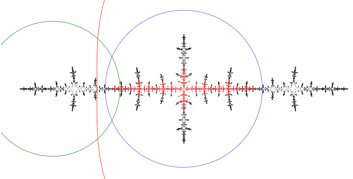
    On the picture below the central U' region (limited by the blue circle) is mapped by the f-1 twice to the left (inside the green circle). Then the circle is mapped one-to-one (quasi-linear) into the U region (inside the red curve). That is the whole f-1o2 map from U' to U is quadratic-like.

    Controls: Drag the blue circle to change its radius. Click mouse + <Alt>/<Ctrl> to zoom In/Out.

    5.2.1.png
    Figure \(\PageIndex{1}\)

    The inverse fc-2(z) map has four branches (see Iterations of inverse maps)

        ±(±(z - c)½ - c)½.

    To get the green circle from the red U region we shall take -(z - c)½, therefore the whole inverse quadratic-like map is

        fc-2(z) = ±(-(z - c)½ - c)½.

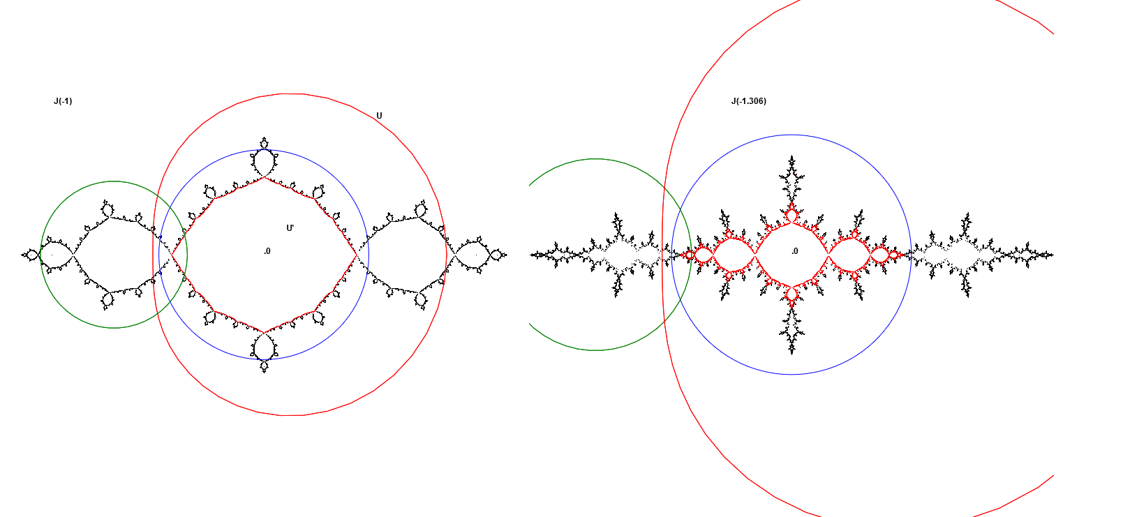
    Iterations of this map are shown above in the red color. As since U' lies in U, therefore iterations of a point in U stay in U' forever and we get the renormalized Julia set homeomorphic to J(0) (i.e. a circle). To the right you see even more impressive the renormalized J(-1) midget inside the J(-1.306) set.

    Renormalization of the J(-1.5438) set below corresponding to the Misiurewicz band merging point is homeomorphic to the J(-2) set (i.e. the straight [-2, 2] segment). J(-1.4304) corresponding to the second band merging point is renormalized in J(-1.5438) (the red midget in the center is equivalent to the whole first picture).

    5.2.2.png
    Figure \(\PageIndex{2}\)
    5.2.3.png
    Figure \(\PageIndex{3}\)


    This page titled 5.2: The Julia set is shared under a Public Domain license and was authored, remixed, and/or curated by via source content that was edited to the style and standards of the LibreTexts platform; a detailed edit history is available upon request.