Section 12.3E: Exercises for Arc Length and Curvature

Determining Arc Length

In questions 1 - 5, find the arc length of the curve on the given interval.

1)  [HW] \(\vecs r(t)=t^2 \,\hat{\mathbf{i}}+(2t^2+1)\,\hat{\mathbf{j}}, \quad 1≤t≤3\)

Answer

\(8\sqrt{5}\) units

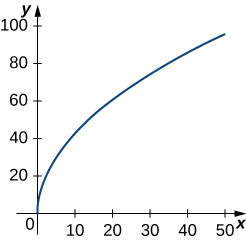
2) \(\vecs r(t)=t^2 \,\hat{\mathbf{i}}+14t \,\hat{\mathbf{j}},\quad 0≤t≤7\). This portion of the graph is shown here:

3) [HW] \(\vecs r(t)=⟨t^2+1,4t^3+3⟩, \quad −1≤t≤0\)

Answer

\(\frac{1}{54}(37^{3/2}−1)\) units

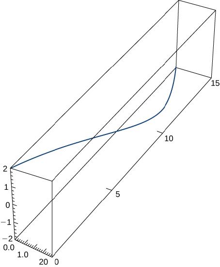
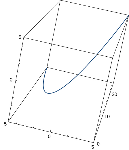
4) [HW] \(\vecs r(t)=⟨2 \sin t,5t,2 \cos t⟩,\quad 0≤t≤π\). This portion of the graph is shown here:

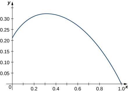
5) \(\vecs r(t)=⟨e^{−t \cos t},e^{−t \sin t}⟩\) over the interval \([0,\frac{π}{2}]\). Here is the portion of the graph on the indicated interval:

6) Set up an integral to represent the arc length from \(t = 0\) to \(t = 2\) along the curve traced out by \(\vecs r(t) = \langle t, \, t^4\rangle.\) Then use technology to approximate this length to the nearest thousandth of a unit.

7) [HW] Find the length of one turn of the helix given by \(\vecs r(t)= \frac{1}{2} \cos t \,\hat{\mathbf{i}}+\frac{1}{2} \sin t \,\hat{\mathbf{j}}+\frac{\sqrt{3}}{2}\,t \,\hat{\mathbf{k}}\).

Answer

Length \(=2π\) units

8) [HW] Find the arc length of the vector-valued function \(\vecs r(t)=−t \,\hat{\mathbf{i}}+4t \,\hat{\mathbf{j}}+3t \,\hat{\mathbf{k}}\) over \([0,1]\). Think of another way to solve this problem, without using an integral. 

9) [HW]  A particle travels in a circle with the equation of motion \(\vecs r(t)=3 \cos t \,\hat{\mathbf{i}}+3 \sin t \,\hat{\mathbf{j}} +0 \,\hat{\mathbf{k}}\). Find the distance traveled around the circle by the particle. Think of another way to solve this problem, without using an integral. 

Answer

\(6π\) units

10) Set up an integral to find the circumference of the ellipse with the equation \(\vecs r(t)= \cos t \,\hat{\mathbf{i}}+2 \sin t \,\hat{\mathbf{j}}+0\,\hat{\mathbf{k}}\).

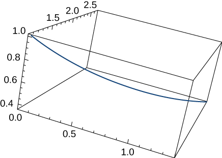
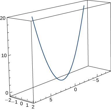
11) [HW] Find the length of the curve \(\vecs r(t)=⟨\sqrt{2}t,\, e^t, \, e^{−t}⟩\) over the interval \(0≤t≤1\). The graph is shown here:

Answer

\(\left(e−\frac{1}{e}\right)\) units

12) Find the length of the curve \(\vecs r(t)=⟨2 \sin t, \, 5t, \, 2 \cos t⟩\) for \(t∈[−10,10]\).

Unit Tangent Vectors and Unit Normal Vectors (optional)

13) The position function for a particle is \(\vecs r(t)=a \cos( ωt) \,\hat{\mathbf{i}}+b \sin (ωt) \,\hat{\mathbf{j}}\). Find the unit tangent vector and the unit normal vector at \(t=0\).

Solution:

\(\begin{align*} \vecs r'(t) &= -aω \sin( ωt) \,\hat{\mathbf{i}}+bω \cos (ωt) \,\hat{\mathbf{j}}\\[5pt]
\| \vecs r'(t) \| &= \sqrt{a^2 ω^2 \sin^2(ωt) +b^2ω^2\cos^2(ωt)} \\[5pt]
\vecs T(t) &= \dfrac{\vecs r'(t)}{\| \vecs r'(t) \| } = \dfrac{-aω \sin( ωt) \,\hat{\mathbf{i}}+bω \cos (ωt) \,\hat{\mathbf{j}}}{\sqrt{a^2 ω^2 \sin^2(ωt) +b^2ω^2\cos^2(ωt)}}\\[5pt]
\vecs T(0) &= \dfrac{bω \,\hat{\mathbf{j}}}{\sqrt{(bω)^2}} = \dfrac{bω \,\hat{\mathbf{j}}}{|bω|}\end{align*}\)

If \(bω > 0, \; \vecs T(0) = \hat{\mathbf{j}},\) and if \( bω < 0, \; T(0)= -\hat{\mathbf{j}}\)

Answer

If \(bω > 0, \; \vecs T(0)= \hat{\mathbf{j}},\) and if \( bω < 0, \; \vecs T(0)= -\hat{\mathbf{j}}\)

If \(a > 0, \; \vecs N(0)= -\hat{\mathbf{i}},\) and if \( a < 0, \; \vecs N(0)= \hat{\mathbf{i}}\)

14) Given \(\vecs r(t)=a \cos (ωt) \,\hat{\mathbf{i}} +b \sin (ωt) \,\hat{\mathbf{j}}\), find the binormal vector \(\vecs B(0)\).

15) Given \(\vecs r(t)=⟨2e^t,e^t \cos t,e^t \sin t⟩\), determine the unit tangent vector \(\vecs T(t)\).

Answer

\(\begin{align*} \vecs T(t) &=\left\langle \frac{2}{\sqrt{6}},\, \frac{\cos t− \sin t}{\sqrt{6}}, \, \frac{\cos t+ \sin t}{\sqrt{6}}\right\rangle \\[4pt]
&= \left\langle\frac{\sqrt{6}}{3},\, \frac{\sqrt{6}}{6} (\cos t− \sin t), \, \frac{\sqrt{6}}{6} (\cos t+ \sin t)\right\rangle \end{align*}\)

16) Given \(\vecs r(t)=⟨2e^t,\, e^t \cos t,\, e^t \sin t⟩\), find the unit tangent vector \(\vecs T(t)\) evaluated at \(t=0\), \(\vecs T(0)\).

17) Given \(\vecs r(t)=⟨2e^t,\, e^t \cos t,\, e^t \sin t⟩\), determine the unit normal vector \(\vecs N(t)\).

Answer

\(\vecs N(t)=⟨0,\, -\frac{\sqrt{2}}{2} (\sin t + \cos t), \, \frac{\sqrt{2}}{2} (\cos t- \sin t)⟩\)

18) Given \(\vecs r(t)=⟨2e^t,\, e^t \cos t,\, e^t \sin t⟩\), find the unit normal vector \(\vecs N(t)\) evaluated at \(t=0\), \(\vecs N(0)\).

Answer

\(\vecs N(0)=⟨0, \;-\frac{\sqrt{2}}{2},\;\frac{\sqrt{2}}{2}⟩\)

19) Given \(\vecs r(t)=t \,\hat{\mathbf{i}}+t^2 \,\hat{\mathbf{j}}+t \,\hat{\mathbf{k}}\), find the unit tangent vector \(\vecs T(t)\). The graph is shown here:

Answer

\(\vecs T(t)=\dfrac{1}{\sqrt{4t^2+2}}<1,2t,1>\)

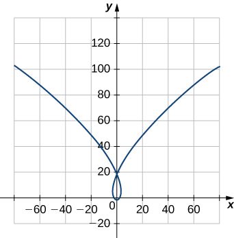
20) Find the unit tangent vector \(\vecs T(t)\) and unit normal vector \(\vecs N(t)\) at \(t=0\) for the plane curve \(\vecs r(t)=⟨t^3−4t,5t^2−2⟩\). The graph is shown here:

21) Find the unit tangent vector \(\vecs T(t)\) for \(\vecs r(t)=3t \,\hat{\mathbf{i}}+5t^2 \,\hat{\mathbf{j}}+2t \,\hat{\mathbf{k}}\).

Answer

\(\vecs T(t)=\dfrac{1}{\sqrt{100t^2+13}}(3 \,\hat{\mathbf{i}}+10t \,\hat{\mathbf{j}}+2 \,\hat{\mathbf{k}})\)

22) Find the principal normal vector to the curve \(\vecs r(t)=⟨6 \cos t,6 \sin t⟩\) at the point determined by \(t=\frac{π}{3}\).

23) Find \(\vecs T(t)\) for the curve \(\vecs r(t)=(t^3−4t) \,\hat{\mathbf{i}}+(5t^2−2) \,\hat{\mathbf{j}}\).

Answer

\(\vecs T(t)=\dfrac{1}{\sqrt{9t^4+76t^2+16}}\big((3t^2−4)\,\hat{\mathbf{i}}+10t \,\hat{\mathbf{j}}\big)\)

24) Find \(\vecs N(t)\) for the curve \(\vecs r(t)=(t^3−4t)\,\hat{\mathbf{i}}+(5t^2−2)\,\hat{\mathbf{j}}\).

25) Find the unit tangent vector \(\vecs T(t)\) for \(\vecs r(t)=⟨2 \sin t,\, 5t,\, 2 \cos t⟩\).

Answer

\(\vecs T(t)=⟨\frac{2\sqrt{29}}{29}\cos t,\, \frac{5\sqrt{29}}{29},\,−\frac{2\sqrt{29}}{29}\sin t⟩\)

26) Find the unit normal vector \(\vecs N(t)\) for \(\vecs r(t)=⟨2\sin t,\,5t,\,2\cos t⟩\).

Answer

\(\vecs N(t)=⟨−\sin t,\, 0,\, −\cos t⟩\)

Arc Length Parameterizations (optional)

27) Find the arc-length function \(\vecs s(t)\) for the line segment given by \(\vecs r(t)=⟨3−3t,\, 4t⟩\). Then write the arc-length parameterization of \(r\) with \(s\) as the parameter.

Answer

Arc-length function: \(s(t)=5t\); The arc-length parameterization of \(\vecs r(t)\): \(\vecs r(s)=\left(3−\dfrac{3s}{5}\right)\,\hat{\mathbf{i}}+\dfrac{4s}{5}\,\hat{\mathbf{j}}\)

28) Parameterize the helix \(\vecs r(t)= \cos t \,\hat{\mathbf{i}}+ \sin t \,\hat{\mathbf{j}}+t \,\hat{\mathbf{k}}\) using the arc-length parameter \(s\), from \(t=0\).

29) Parameterize the curve using the arc-length parameter \(s\), at the point at which \(t=0\) for \(\vecs r(t)=e^t \sin t \,\hat{\mathbf{i}} + e^t \cos t \,\hat{\mathbf{j}}\)

Answer

\(\vecs r(s)=\left(1+\dfrac{s}{\sqrt{2}}\right) \sin \left( \ln \left(1+ \dfrac{s}{\sqrt{2}}\right)\right)\,\hat{\mathbf{i}} +\left(1+ \dfrac{s}{\sqrt{2}}\right) \cos \left( \ln \left(1+\dfrac{s}{\sqrt{2}}\right)\right)\,\hat{\mathbf{j}}\)

Curvature and the Osculating Circle (optional)

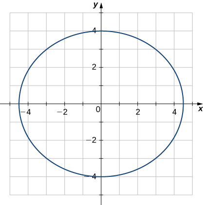
30) Find the curvature of the curve \(\vecs r(t)=5 \cos t \,\hat{\mathbf{i}}+4 \sin t \,\hat{\mathbf{j}}\) at \(t=π/3\). (Note: The graph is an ellipse.)

31) Find the \(x\)-coordinate at which the curvature of the curve \(y=1/x\) is a maximum value.

Answer

The maximum value of the curvature occurs at \(x=1\).

32) Find the curvature of the curve \(\vecs r(t)=5 \cos t \,\hat{\mathbf{i}}+5 \sin t \,\hat{\mathbf{j}}\). Does the curvature depend upon the parameter \(t\)?

33) Find the curvature \(κ\) for the curve \(y=x−\frac{1}{4}x^2\) at the point \(x=2\).

Answer

\(\frac{1}{2}\)

34) Find the curvature \(κ\) for the curve \(y=\frac{1}{3}x^3\) at the point \(x=1\).

35) Find the curvature \(κ\) of the curve \(\vecs r(t)=t \,\hat{\mathbf{i}}+6t^2 \,\hat{\mathbf{j}}+4t \,\hat{\mathbf{k}}\). The graph is shown here:

Answer

\(κ≈\dfrac{49.477}{(17+144t^2)^{3/2}}\)

36) Find the curvature of \(\vecs r(t)=⟨2 \sin t,5t,2 \cos t⟩\).

37) Find the curvature of \(\vecs r(t)=\sqrt{2}t \,\hat{\mathbf{i}}+e^t \,\hat{\mathbf{j}}+e^{−t} \,\hat{\mathbf{k}}\) at point \(P(0,1,1)\).

Answer

\(\frac{1}{2\sqrt{2}}\)

38) At what point does the curve \(y=e^x\) have maximum curvature?

39) What happens to the curvature as \(x→∞\) for the curve \(y=e^x\)?

Answer

The curvature approaches zero.

40) Find the point of maximum curvature on the curve \(y=\ln x\).

41) Find the equations of the normal plane and the osculating plane of the curve \(\vecs r(t)=⟨2 \sin (3t),t,2 \cos (3t)⟩\) at point \((0,π,−2)\).

Answer

\(y=6x+π\) and \(x+6y=6π\)

42) Find equations of the osculating circles of the ellipse \(4y^2+9x^2=36\) at the points \((2,0)\) and \((0,3)\).

43) Find the equation for the osculating plane at point \(t=π/4\) on the curve \(\vecs r(t)=\cos (2t) \,\hat{\mathbf{i}}+ \sin (2t) \,\hat{\mathbf{j}}+t\,\hat{\mathbf{k}}\).

Answer

\(x+2z=\frac{π}{2}\)

44) Find the radius of curvature of \(6y=x^3\) at the point \((2,\frac{4}{3}).\)

45) Find the curvature at each point \((x,y)\) on the hyperbola \(\vecs r(t)=⟨a \cosh( t),b \sinh (t)⟩\).

Answer

\(\dfrac{a^4b^4}{(b^4x^2+a^4y^2)^{3/2}}\)

46) Calculate the curvature of the circular helix \(\vecs r(t)=r \sin (t) \,\hat{\mathbf{i}}+r \cos (t) \,\hat{\mathbf{j}}+t \,\hat{\mathbf{k}}\).

47) Find the radius of curvature of \(y= \ln (x+1)\) at point \((2,\ln 3)\).

Answer

\(\frac{10\sqrt{10}}{3}\)

48) Find the radius of curvature of the hyperbola \(xy=1\) at point \((1,1)\).

A particle moves along the plane curve \(C\) described by \(\vecs r(t)=t \,\hat{\mathbf{i}}+t^2 \,\hat{\mathbf{j}}\). Use this parameterization to answer questions 49 - 51.

49) Find the length of the curve over the interval \([0,2]\).

Answer

\(\frac{1}{4}\big[ 4\sqrt{17} + \ln\left(4+\sqrt{17}\right)\big]\text{ units }\approx 4.64678 \text{ units}\)

50) Find the curvature of the plane curve at \(t=0,1,2\).

51) Describe the curvature as t increases from \(t=0\) to \(t=2\).

Answer

The curvature is decreasing over this interval.

The surface of a large cup is formed by revolving the graph of the function \(y=0.25x^{1.6}\) from \(x=0\) to \(x=5\) about the \(y\)-axis (measured in centimeters).

52) [T] Use technology to graph the surface.

53) Find the curvature \(κ\) of the generating curve as a function of \(x\).

Answer

\(κ=\dfrac{30}{x^{2/5}\left(25+4x^{6/5}\right)^{3/2}}\)

Note that initially your answer may be:
\(\dfrac{6}{25x^{2/5}\left(1+\frac{4}{25}x^{6/5}\right)^{3/2}}\)

We can simplify it as follows:
\( \begin{align*} \dfrac{6}{25x^{2/5}\left(1+\frac{4}{25}x^{6/5}\right)^{3/2}} &= \dfrac{6}{25x^{2/5}\big[\frac{1}{25}\left(25+4x^{6/5}\right)\big]^{3/2}}\\[4pt]
&= \dfrac{6}{25x^{2/5}\left(\frac{1}{25}\right)^{3/2}\big[25+4x^{6/5}\big]^{3/2}} \\[4pt]
&= \dfrac{6}{\frac{25}{125}x^{2/5}\big[25+4x^{6/5}\big]^{3/2}} \\[4pt]
&= \dfrac{30}{x^{2/5}\left(25+4x^{6/5}\right)^{3/2}}\end{align*} \)

54) [T] Use technology to graph the curvature function.

Contributors:

• Gilbert Strang (MIT) and Edwin “Jed” Herman (Harvey Mudd) with many contributing authors. This content by OpenStax is licensed with a CC-BY-SA-NC 4.0 license. Download for free at http://cnx.org.

• Paul Seeburger (Monroe Community College) created question 6.