2.3: Integration

Finding Area

Let's use a Monte-Carlo type method to calculate area. Suppose we have the following circular dart board and want to know its area.

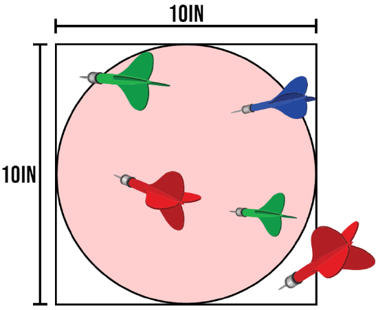
We enclose the dart board with a square of known area, in this case 100in², and perform following the following procedure:

1. Throw darts at the square, being careful not to favor any particular spot.
2. Record the percentage of darts that land inside the circle.
3. Multiply this percentage by the known area of the square (100in²)
4. That's our approximation!

Of course, doing this by hand would take a lot of time. Instead, we can use Python. In our program, we will randomly choose an x-value and y-value using the random.uniform(start,stop) function. This function returns a random float in [start,stop). We will center our circle at the origin, so we will use random.uniform(-5,5) for both the x and y values.

Next, we need to have a way to determine whether the point (x,y) lies inside the circle or not. We know that the equation of the circle under discussion will be

\[x^2+y^2=5^2\]

Solving for \(y\), we get

\[y=\pm\sqrt{25-x^2}.\]

Thus, in our python code, we will check that

\[y\leq\sqrt{25-x^2}\hspace{10pt}\textrm{     and     }\hspace{10pt}y\geq-\sqrt{25-x^2}.\]

That is, that it is below the top half of the circle and above the bottom half of the circle. Here we go!

import random

tries=10000
success=0
for a in range(1,tries+1):
  x=random.uniform(-5,5)
  y=random.uniform(-5,5)
  if (y<=(25-x**2)**(1/2)) and (y>=-(25-x**2)**(1/2)):
    success+=1
print(100*success/tries)

output:     78.52

Above, the percentage of "darts" that hit the circle is given by success/tries. We then multiplied that by the area of the square (100) to get the approximate area of the circle, which is given as 78.52, very close to our expected value of \(25\pi\).

For fun, we could plot each of the dots to see what our board looks like. Here is an example with 100 dots:

import random
import numpy as np
import matplotlib.pyplot as plt
 
xc = np.linspace(-5, 5, 1000)
yc = (25-xc**2)**(1/2)
zc = -(25-xc**2)**(1/2)
plt.plot(xc, yc, color='red', linewidth=2.0, linestyle='-')
plt.plot(xc, zc, color='red', linewidth=2.0, linestyle='-')

#we need to make the axes have the same scale so it looks like a circle.
#these two lines do that.
ax = plt.gca()
ax.set_aspect('equal', adjustable='box')

tries=100
success=0
for a in range(1,tries+1):
  x=random.uniform(-5,5)
  y=random.uniform(-5,5)
  if (y<=(25-x**2)**(1/2)) and (y>=-(25-x**2)**(1/2)):
    success+=1
  plt.plot(x,y,'o',color='black')
print(100*success/tries)
plt.show()

output:     80

Integrals

Now that we've found area using a Monte-Carlo type simulation, you might have an idea of how to calculate integrals: just find the area under the curve!

Example: Use a Monte-Carlo type simulation to find the area under the curve over \([0,4]\)

\[y=0.5x^2\]

Answer: To start, we need to find a box that will fit the entire curve we are calculating. The x-values are easy: just use the given interval \([0,4]\). For the y-values, we need to find the least and greatest y-values that this curve achieves. Since this is a parabola, we can see that the least y-value is 0 and the greatest is \(0.5*(4)^2=8\). So our box will be \([0,4]x[0,8]\). That means our random points will have x-values in [0,4] and y-values in [0,8]. We will determine whether the point is above or below the curve similar to the circle example above. We will consider a "success" - that is, consider our point to be under the curve - if:

\[y\leq 0.5x^2.\]

Note that we don't need to determine whether the point is above the x-axis because our y-values are only chosen from [0,8]. The area of our box is 4*8=32. Let's modify the above program:

import random
import numpy as np
import matplotlib.pyplot as plt
 
xc = np.linspace(0, 4, 1000)
yc = 0.5*xc**2
plt.plot(xc, yc, color='red', linewidth=2.0, linestyle='-')

tries=1000
success=0
for a in range(1,tries+1):
  x=random.uniform(0,4)
  y=random.uniform(0,8)
  if (y<=(0.5*x**2)):
    success+=1
  plt.plot(x,y,'o',color='black')
print(32*success/tries)
plt.show()

output:     10.208

This is relatively close to our expected value (using integration) of 10.6667. If we increase the "tries" variable, we can get even closer. However, this will make our picture look like a blob!

Exercise

Use the techniques above to approximate the integral \[\int_{\pi/2}^\pi\]

1. \(11\)
2. \(3\)
3. \(-4\)

Answer

1. \(\frac{11}{1}\)
2. \(\frac{3}{1}\)
3. \(-\frac{4}{1}\)