Mathematics LibreTexts

3.1: Introduction to Interpolation and Curve Fitting

  • Page ID
    122392
  • \( \newcommand{\vecs}[1]{\overset { \scriptstyle \rightharpoonup} {\mathbf{#1}} } \)

    \( \newcommand{\vecd}[1]{\overset{-\!-\!\rightharpoonup}{\vphantom{a}\smash {#1}}} \)

    \( \newcommand{\id}{\mathrm{id}}\) \( \newcommand{\Span}{\mathrm{span}}\)

    ( \newcommand{\kernel}{\mathrm{null}\,}\) \( \newcommand{\range}{\mathrm{range}\,}\)

    \( \newcommand{\RealPart}{\mathrm{Re}}\) \( \newcommand{\ImaginaryPart}{\mathrm{Im}}\)

    \( \newcommand{\Argument}{\mathrm{Arg}}\) \( \newcommand{\norm}[1]{\| #1 \|}\)

    \( \newcommand{\inner}[2]{\langle #1, #2 \rangle}\)

    \( \newcommand{\Span}{\mathrm{span}}\)

    \( \newcommand{\id}{\mathrm{id}}\)

    \( \newcommand{\Span}{\mathrm{span}}\)

    \( \newcommand{\kernel}{\mathrm{null}\,}\)

    \( \newcommand{\range}{\mathrm{range}\,}\)

    \( \newcommand{\RealPart}{\mathrm{Re}}\)

    \( \newcommand{\ImaginaryPart}{\mathrm{Im}}\)

    \( \newcommand{\Argument}{\mathrm{Arg}}\)

    \( \newcommand{\norm}[1]{\| #1 \|}\)

    \( \newcommand{\inner}[2]{\langle #1, #2 \rangle}\)

    \( \newcommand{\Span}{\mathrm{span}}\) \( \newcommand{\AA}{\unicode[.8,0]{x212B}}\)

    \( \newcommand{\vectorA}[1]{\vec{#1}}      % arrow\)

    \( \newcommand{\vectorAt}[1]{\vec{\text{#1}}}      % arrow\)

    \( \newcommand{\vectorB}[1]{\overset { \scriptstyle \rightharpoonup} {\mathbf{#1}} } \)

    \( \newcommand{\vectorC}[1]{\textbf{#1}} \)

    \( \newcommand{\vectorD}[1]{\overrightarrow{#1}} \)

    \( \newcommand{\vectorDt}[1]{\overrightarrow{\text{#1}}} \)

    \( \newcommand{\vectE}[1]{\overset{-\!-\!\rightharpoonup}{\vphantom{a}\smash{\mathbf {#1}}}} \)

    \( \newcommand{\vecs}[1]{\overset { \scriptstyle \rightharpoonup} {\mathbf{#1}} } \)

    \( \newcommand{\vecd}[1]{\overset{-\!-\!\rightharpoonup}{\vphantom{a}\smash {#1}}} \)

    Given a set of data, we might want to approximate the value in between, after, or before what is given. To do this, we can generate a curve by using either interpolation or curve fitting. Interpolation is a method of estimating the value of a function at a given point within the range of a set of known data points. It involves finding a polynomial that fits a set of data points exactly, rather than just approximating them. Curve fitting, on the other hand, is the process of finding the best-fitting curve, where the goal is to find a model that captures the underlying trends in the data, rather than fitting the data points exactly.

    For example, suppose we are given the following data points. Perhaps this data represents the temperature over several days, or the location of a board over the past several hours. We are wanting to estimate what the temperature was - or where the boat was - in between data points D and E.
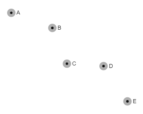
     

    clipboard_e0aa238b261f9856b0d6f823bed0d9598.png

    A discrete data set


    To do this, we first use interpolation, that is, generate a polynomial that exactly matches the data set. In general, if we are using interpolation on \(n\) points, we can use a polynomial of degree \(n-1\). In this case, we will use a polynomial of degree 4.


    clipboard_e0aa238b261f9856b0d6f823bed0d9598.png

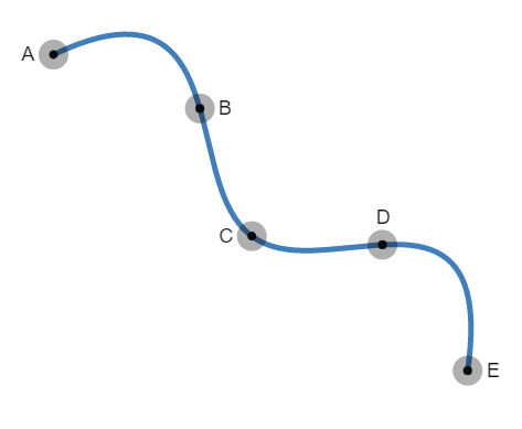
    Example of Interpolation

    Your intuition might say that this is an unusual path for temperature to follow, though maybe it makes sense for the drifting of a boat. Either way, let's next fit a line to the data set.


    clipboard_e0aa238b261f9856b0d6f823bed0d9598.png

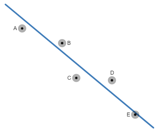
    Example of Curve Fitting

    In the sections that follow, we find techniques to generate these curves in the best possible way.


    3.1: Introduction to Interpolation and Curve Fitting is shared under a CC BY-NC-SA license and was authored, remixed, and/or curated by LibreTexts.

    • Was this article helpful?