3.2: Polynomial Interpolation

Last updated

Feb 9, 2023
Save as PDF
- 3.1: Introduction to Interpolation and Curve Fitting
- Back Matter

$\newcommand{\vecs}[1]{\overset { \scriptstyle \rightharpoonup} {\mathbf{#1}} }$

$\newcommand{\vecd}[1]{\overset{-\!-\!\rightharpoonup}{\vphantom{a}\smash {#1}}}$

$\newcommand{\id}{\mathrm{id}}$ $\newcommand{\Span}{\mathrm{span}}$

( \newcommand{\kernel}{\mathrm{null}\,}\) $\newcommand{\range}{\mathrm{range}\,}$

$\newcommand{\RealPart}{\mathrm{Re}}$ $\newcommand{\ImaginaryPart}{\mathrm{Im}}$

$\newcommand{\Argument}{\mathrm{Arg}}$ $\newcommand{\norm}[1]{\| #1 \|}$

$\newcommand{\inner}[2]{\langle #1, #2 \rangle}$

$\newcommand{\Span}{\mathrm{span}}$

$\newcommand{\id}{\mathrm{id}}$

$\newcommand{\Span}{\mathrm{span}}$

$\newcommand{\kernel}{\mathrm{null}\,}$

$\newcommand{\range}{\mathrm{range}\,}$

$\newcommand{\RealPart}{\mathrm{Re}}$

$\newcommand{\ImaginaryPart}{\mathrm{Im}}$

$\newcommand{\Argument}{\mathrm{Arg}}$

$\newcommand{\norm}[1]{\| #1 \|}$

$\newcommand{\inner}[2]{\langle #1, #2 \rangle}$

$\newcommand{\Span}{\mathrm{span}}$ $\newcommand{\AA}{\unicode[.8,0]{x212B}}$

$\newcommand{\vectorA}[1]{\vec{#1}} % arrow$

$\newcommand{\vectorAt}[1]{\vec{\text{#1}}} % arrow$

$\newcommand{\vectorB}[1]{\overset { \scriptstyle \rightharpoonup} {\mathbf{#1}} }$

$\newcommand{\vectorC}[1]{\textbf{#1}}$

$\newcommand{\vectorD}[1]{\overrightarrow{#1}}$

$\newcommand{\vectorDt}[1]{\overrightarrow{\text{#1}}}$

$\newcommand{\vectE}[1]{\overset{-\!-\!\rightharpoonup}{\vphantom{a}\smash{\mathbf {#1}}}}$

$\newcommand{\vecs}[1]{\overset { \scriptstyle \rightharpoonup} {\mathbf{#1}} }$

$\newcommand{\vecd}[1]{\overset{-\!-\!\rightharpoonup}{\vphantom{a}\smash {#1}}}$

$\newcommand{\avec}{\mathbf a}$

$\newcommand{\bvec}{\mathbf b}$

$\newcommand{\cvec}{\mathbf c}$

$\newcommand{\dvec}{\mathbf d}$

$\newcommand{\dtil}{\widetilde{\mathbf d}}$

$\newcommand{\evec}{\mathbf e}$

$\newcommand{\fvec}{\mathbf f}$

$\newcommand{\nvec}{\mathbf n}$

$\newcommand{\pvec}{\mathbf p}$

$\newcommand{\qvec}{\mathbf q}$

$\newcommand{\svec}{\mathbf s}$

$\newcommand{\tvec}{\mathbf t}$

$\newcommand{\uvec}{\mathbf u}$

$\newcommand{\vvec}{\mathbf v}$

$\newcommand{\wvec}{\mathbf w}$

$\newcommand{\xvec}{\mathbf x}$

$\newcommand{\yvec}{\mathbf y}$

$\newcommand{\zvec}{\mathbf z}$

$\newcommand{\rvec}{\mathbf r}$

$\newcommand{\mvec}{\mathbf m}$

$\newcommand{\zerovec}{\mathbf 0}$

$\newcommand{\onevec}{\mathbf 1}$

$\newcommand{\real}{\mathbb R}$

$\newcommand{\twovec}[2]{\left[\begin{array}{r}#1 \\ #2 \end{array}\right]}$

$\newcommand{\ctwovec}[2]{\left[\begin{array}{c}#1 \\ #2 \end{array}\right]}$

$\newcommand{\threevec}[3]{\left[\begin{array}{r}#1 \\ #2 \\ #3 \end{array}\right]}$

$\newcommand{\cthreevec}[3]{\left[\begin{array}{c}#1 \\ #2 \\ #3 \end{array}\right]}$

$\newcommand{\fourvec}[4]{\left[\begin{array}{r}#1 \\ #2 \\ #3 \\ #4 \end{array}\right]}$

$\newcommand{\cfourvec}[4]{\left[\begin{array}{c}#1 \\ #2 \\ #3 \\ #4 \end{array}\right]}$

$\newcommand{\fivevec}[5]{\left[\begin{array}{r}#1 \\ #2 \\ #3 \\ #4 \\ #5 \\ \end{array}\right]}$

$\newcommand{\cfivevec}[5]{\left[\begin{array}{c}#1 \\ #2 \\ #3 \\ #4 \\ #5 \\ \end{array}\right]}$

$\newcommand{\mattwo}[4]{\left[\begin{array}{rr}#1 \amp #2 \\ #3 \amp #4 \\ \end{array}\right]}$

$\newcommand{\laspan}[1]{\text{Span}\{#1\}}$

$\newcommand{\bcal}{\cal B}$

$\newcommand{\ccal}{\cal C}$

$\newcommand{\scal}{\cal S}$

$\newcommand{\wcal}{\cal W}$

$\newcommand{\ecal}{\cal E}$

$\newcommand{\coords}[2]{\left\{#1\right\}_{#2}}$

$\newcommand{\gray}[1]{\color{gray}{#1}}$

$\newcommand{\lgray}[1]{\color{lightgray}{#1}}$

$\newcommand{\rank}{\operatorname{rank}}$

$\newcommand{\row}{\text{Row}}$

$\newcommand{\col}{\text{Col}}$

$\renewcommand{\row}{\text{Row}}$

$\newcommand{\nul}{\text{Nul}}$

$\newcommand{\var}{\text{Var}}$

$\newcommand{\corr}{\text{corr}}$

$\newcommand{\len}[1]{\left|#1\right|}$

$\newcommand{\bbar}{\overline{\bvec}}$

$\newcommand{\bhat}{\widehat{\bvec}}$

$\newcommand{\bperp}{\bvec^\perp}$

$\newcommand{\xhat}{\widehat{\xvec}}$

$\newcommand{\vhat}{\widehat{\vvec}}$

$\newcommand{\uhat}{\widehat{\uvec}}$

$\newcommand{\what}{\widehat{\wvec}}$

$\newcommand{\Sighat}{\widehat{\Sigma}}$

$\newcommand{\lt}{<}$

$\newcommand{\gt}{>}$

$\newcommand{\amp}{&}$

$\definecolor{fillinmathshade}{gray}{0.9}$

Given a set of data, polynomial interpolation is a method of finding a polynomial function that fits a set of data points exactly. Though there are several methods for finding this polynomial, the polynomial itself is unique, which we will prove later.

3.2.1: Lagrange Polynomial

One of the most common ways to perform polynomial interpolation is by using the Lagrange polynomial. To motivate this method, we begin by constructing a polynomial that goes through 2 data points $(x_0,y_0)$ and $x_1,y_1$ . We use two equations from college algebra.

$y-y_1=m(x-x_1)\hspace{10pt}\textrm{and}\hspace{10pt}m=\frac{y_1-y_0}{x_1-x_0}$

Combining these, we end up with:

$y=\frac{y_1-y_0}{x_1-x_0}(x-x_1)+y_1.$

Now, to derive a formula similar to that used for the Lagrange polynomial, we perform some algebra. We begin by swapping the terms $y_1-y_0$ and $x-x_1$ :

$y=\frac{x-x_1}{x_1-x_0}(y_1-y_0)+y_1.$

Distributing the fraction:

$y=\frac{x-x_1}{x_1-x_0}y_1 - \frac{x-x_1}{x_1-x_0}y_0 + y_1.$

Multiplying the right-most $y_1$ term by $\frac{x_1-x_0}{x_1-x_0}=1$ :

$y=\frac{x-x_1}{x_1-x_0}y_1 - \frac{x-x_1}{x_1-x_0}y_0 + \frac{x_1-x_0}{x_1-x_0}y_1.$

Combining to the $y_1$ terms:

$y=-\frac{x-x_1}{x_1-x_0}y_0 + \frac{x-x_0}{x_1-x_0}y_1.$

and finally flipping the denominator of the first term to get rid of the negative:

$y=\frac{x-x_1}{x_0-x_1}y_0 + \frac{x-x_0}{x_1-x_0}y_1.$

In the above, we can observe that, when $x=x_1$ , it follows that the first term cancels out with a zero on top and the second term ends up as $1\cdot y_1=y_1$ , as desired. Similarly, if $x=x_0$ , then the first term ends up as $1\cdot y_0=y_0$ and the second term cancels out with a zero on top, causing the entire expression to be $y_0$ , as desired.

For three data points $(x_0,y_0), (x_1,y_1), \textrm{and} (x_2,y_2),$ we can derive a polynomial that behaves similarly:

$y=\frac{(x-x_1)(x-x_2)}{(x_0-x_1)(x_0-x_2)}y_0 + \frac{(x-x_0)(x-x_2)}{(x_1-x_0)(x_1-x_2)}y_1 + \frac{(x-x_0)(x-x_1)}{(x_2-x_0)(x_2-x_1)}y_2.$

In the above, plugging in, for example, $x=x_1$ has the first and third terms cancelling out with zero and the middle term turning into $1\cdot y_1$ , as desired. We can follow this pattern to arrive at the full Lagrange polynomial.

THE LAGRANGE POLYNOMIAL

Given

$n+1$ data points

$(x_0,y_0), (x_1,y_1), \ldots, (x_n,y_n)$ with

$x_0<x_1<\cdots<x_n$ , the Lagrange polynomial is the

$n$ th degree polynomial passing through each of these points and written as:

$y=\frac{(x-x_1)(x-x_2)\cdots(x-x_n)}{(x_0-x_1)(x_0-x_2)\cdots (x_0-x_n)}y_0 + \frac{(x-x_0)(x-x_2)\cdots(x-x_n)}{(x_1-x_0)(x_1-x_2)\cdots (x_1-x_n)}y_1 + \cdots + \frac{(x-x_0)(x-x_1)\cdots(x-x_{n-1})}{(x_n-x_0)(x_n-x_1)\cdots (x_n-x_{n-1})}y_n$ Equivalently, we can use product notation:

$y=\sum_{i=0}^n\left(y_i\prod_{\substack{j=0 \\ j\neq i}}^n\frac{x-x_j}{x_i-x_j}\right)$

Note that in the above polynomial, each numerator is written such that, for $x=x_i$ , each coefficient vanishes except for the coefficient to $y_i$ , which evaluates to $y_i$ . Thus the above polynomial passes through each of the desired data points and, as can be checked, is of degree $n$ .

Now, let's work with Python. To do this, we use function blocks for the first time. We have used functions in the past in Python, such as sin(x) or cos(x). Here, we create our own function using the def keyword. Below, we define f(o), where o is the dynamic variable. At the end of a function block, we "return", using the return keyword, the result of the function calculation. In the code below, the variable o represents the variable x in the Lagrange Polynomial definition above. We do this since x is already used for our data points.

01import numpy as np
02import matplotlib.pyplot as plot
03 
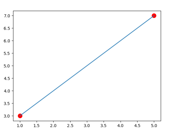
04#Data goes through the points (1,3) and (5,7)
05x=[1,5]
06y=[3,7]
07 
08#Set the number of data points
09pts=len(x)-1
10prange=np.linspace(x[0],x[pts],50)
11 
12plot.plot(x,y,marker='o', color='r', ls='',markersize=10)
13 
14def f(o):
15    z=((o-x[1])/(x[0]-x[1]))*y[0] + ((o-x[0])/(x[1]-x[0]))*y[1]
16    return z
17 
18plot.plot(prange,f(prange))
19plot.show()

output:

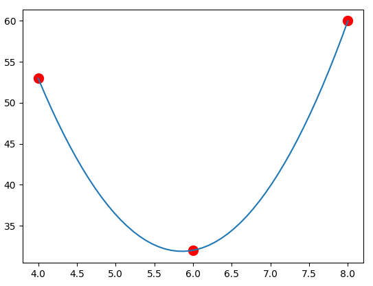
Now, we do the same as the above except with 3 data points. Notice how the only changes are the data point lists and the function. Below, we again use the "\" symbol to let Python know to continue on the next line. This is done to make the polynomial easier to read.

01import numpy as np
02import matplotlib.pyplot as plot
03 
04#data goes through the points (4,1), (6,1) and (8,0)
05x=[4,6,8]
06y=[53,32,60]
07 
08n=len(x)-1
09prange = np.linspace(x[0],x[n],50)
10 
11plot.plot(x,y,marker='o', color='r', ls='', markersize=10)
12 
13def f(o):
14  z=\
15  (((o-x[1])*(o-x[2]))/((x[0]-x[1])*(x[0]-x[2])))*y[0]+\
16  (((o-x[0])*(o-x[2]))/((x[1]-x[0])*(x[1]-x[2])))*y[1]+\
17  (((o-x[0])*(o-x[1]))/((x[2]-x[0])*(x[2]-x[1])))*y[2]
18  return z
19 
20plot.plot(prange,f(prange))
21plot.show()

output:

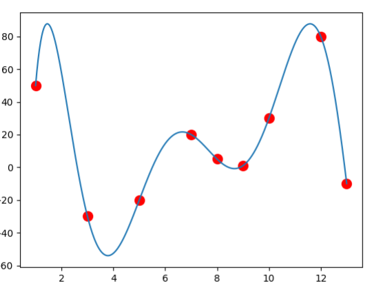
Using the product notation of Lagrange Polynomials, we can even come up with a program that accepts any number of data points.

$y=\sum_{i=0}^n\left(y_i\prod_{\substack{j=0 \\ j\neq i}}^n\frac{x-x_j}{x_i-x_j}\right)$ In the code below,

$i$ and

$j$ represent the

$i$ and

$j$ in the definition above.

01import numpy as np
02import matplotlib.pyplot as plot
03 
04x=[1,3,5,7,8,9,10,12,13]
05y=[50,-30,-20,20,5,1,30,80,-10]
06 
07n=len(x)-1
08prange = np.linspace(min(x),max(x),500)
09 
10plot.plot(x,y,marker='o', color='r', ls='', markersize=10)
11 
12def f(o):
13  sum = 0
14  for i in range(n+1):
15    prod = y[i]
16    for j in range(n+1):
17      if i!= j:
18        prod=prod*(o-x[j])/(x[i]-x[j])
19    sum = sum + prod
20  return sum
21 
22plot.plot(prange,f(prange))
23plot.show()

output:

While Lagrange polynomials are among the easiest methods to understand intuitively and are efficient for calculating a specific $y(x)$ , they fail when when attempting to either find an explicit formula $y=a_0+a_1x+\cdots+a_nx^n$ or when performing incremental interpolation, that is, adding data points after the initial interpolation is performed. For incremental interpolation, we would need to complete re-perform the entire evaluation.

3.2.2: Newton interpolation

Newton interpolation is an alternative to the Lagrange polynomial. Though it appears more cryptic, it allows for incremental interpolation and provides an efficient way to find an explicit formula $y=a_0+a_1x+\cdots+a_nx^n$ .

Newton interpolation is all about finding coefficients and then using those coefficients to calculate subsequent coefficients. Since an important part of Newton interpolation is that it can be used for incremental interpolation, let's start with a single data point and show the calculations as we add points.

With one data point $(x_0,y_0)$ , the calculation is simple:

$b_0=y_0$

and the polynomial is

$y=b_0.$

Let's add a new data point $(x_1,y_1)$ . The next coefficient $b_1$ is usually denoted by $[y_0,y_1]$ :

$b_1=[y_0,y_1]=\frac{y_1-y_0}{x_1-x_0}$

and the polynomial is

$y=b_0+b_1(x-x_0).$

Notice how we did not have to re-calculate the entire polynomial, only the new coefficient to $(x-x_0)$ .

With a third data point $(x_2,y_2)$ , we find the coefficient $b_2=[y_0,y_1,y_2]$ :

$b_2=[y_0,y_1,y_2]=\frac{[y_1,y_2]-[y_0,y_1]}{x_2-x_0}=\frac{\frac{y_2-y_1}{x_2-x_1}-\frac{y_1-y_0}{x_1-x_0}}{x_2-x_0}$

with polynomial

$y=b_0+b_1(x-x_0)+b_2(x-x_0)(x-x_1).$

You may have noticed the recursive nature of the previous definitions. This continues for Newton interpolation in general.

NEWTON INTERPOLATION

Given

$n+1$ data points

$(x_0,y_0), (x_1,y_1), \ldots, (x_n,y_n)$ with

$x_0<x_1<\cdots<x_n$ , the Newton interpolation polynomial is the

$n$ th degree polynomial passing through each of these points and written as:

$y=b_0+b_1(x-x_0)+b_2(x-x_0)(x-x_1)+\cdots+b_{n}(x-x_0)(x-x_1)\cdots(x-x_{n-1})$ where

$\begin{align} b_0 &= y_0\\ b_2 &= [y_0,y_1] = \frac{y_1-y_0}{x_1-x_0}\\ b_2 &= [y_0,y_1,y_2] = \frac{\frac{y_2-y_1}{x_2-x_1}-\frac{y_1-y_0}{x_1-x_0}}{x_2-x_0}\\ &\vdots\\ b_{n} &= [y_0, y_2, \ldots, y_n] = \frac{[y_1, y_2, \ldots, y_n] - [y_0, y_1, \ldots, y_{n-1}]}{x_{n}-x_0} \end{align}$

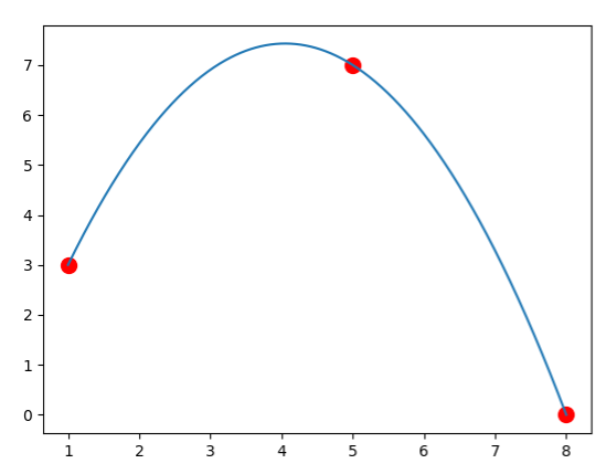
Let's begin by finding a polynomial with three data points using Newton's Method.

Example: Use Newton's method to calculating a polynomial through the points $(1,3), (5,7)$ and $(8,0)$ .

For this example, we will use a "tableau" to help organize our data.

$x_0$	$y_0$
$x_1$	$y_1$	$[y_1,y_0]$
$x_2$	$y_2$	$[y_2,y_1]$	$[y_0,y_1,y_2]$

We start by filling in our data points:

1	3
5	7	$[y_1,y_0]$
8	0	$[y_2,y_1]$	$[y_0,y_1,y_2]$

Then we calculate:

$[y_1,y_0]=\frac{7-3}{5-1}=1$

$[y_2,y_1]=\frac{0-7}{8-5}=-\frac{7}{3}$ and fill in this data:

1	3
5	7	1
8	0	$-\frac{7}{3}$	$[y_0,y_1,y_2]$

Now, we calculate the remaining item, using the previously-calculated terms:

$[y_0,y_1,y_2]=\frac{[y_1,y_2]-[y_0,y_1]}{x_2-x_0}=\frac{-\frac{7}{3}-1}{8-1}=-\frac{10}{21}$

1	3
5	7	1
8	0	$-\frac{7}{3}$	$-\frac{10}{21}$

Note, now, that $b_0, b_1,$ and $b_2$ are written on the top diagonal. Thus our final polynomial is:

$y=b_0+b_1(x-x_0)+b_2(x-x_0)(x-x_1)=3+1(x-1)-\frac{10}{21}(x-1)(x-5)$

Now, let's program this for three data points to check our work!

01import numpy as np
02import matplotlib.pyplot as plot
03 
04x=[1,5,8]
05y=[3,7,0]
06 
07n=len(x)-1
08prange = np.linspace(min(x),max(x),500)
09 
10plot.plot(x,y,marker='o', color='r', ls='', markersize=10)
11 
12def f(o):
13  b0=y[0]
14  b1=(y[1]-y[0])/(x[1]-x[0])
15  b1p=(y[2]-y[1])/(x[2]-x[1])
16  b2=(b1p-b1)/(x[2]-x[0])
17  poly=b0+b1*(o-x[0])+b2*(o-x[0])*(o-x[1])
18  return poly
19 
20plot.plot(prange,f(prange))
21plot.show()

output:

$clipboard_ecc587ffcb22fa6d947d2bb6c5f691ba2.png$

A general program can be made by using a recursive function.

01import numpy as nm
02import matplotlib.pyplot as plot
03 
04x=[-5,-4,-3,-2,-1,0,1,2,3,4,5]
05y=[0,0,0.1,0.3,0.7,1,0.7,0.3,0.1,0,0]
06 
07plot.plot(x,y,marker='o', color='r', ls='',markersize=10)
08 
09def grad(a,b):
10    if a==0: return y[b]
11    return (grad(a-1,b)-grad(a-1,a-1))/(x[b]-x[a-1])
12     
13 
14def f(o):
15    yres=0
16    for p in range(len(x)):
17        prodres=grad(p,p)
18        for q in range(p):
19            prodres*=(o-x[q])
20        yres+=prodres
21    return yres
22prange=nm.linspace(x[0],x[-1],200)
23plot.plot(prange,f(prange))
24plot.show()

output:

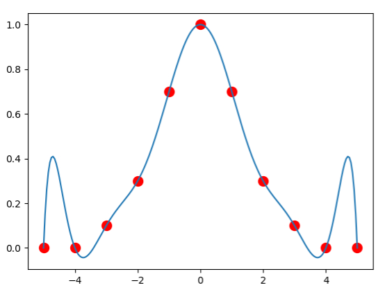
Note that above, we have something strange happening near the end points. This is known as Runge's phenomenon and mainly occurs at the endges of an interval when using polynomial interpolation with polynomials of high degree over a set of points that are equally spaced. Because of Runge's phenomenon, it is often the case that going to higher degrees does not always improve accuracy. To combat this, we can use a method such as cubic splines, which we discuss here.

3.2.3: Cubic Splines

A spline is a function defined piecewise by polynomials. Instead of having a single polynomial that goes through each data point, as we have done so far, we instead define several polynomials between each of the points. While defining several polynomials might take more work, it is usually preferred since it gives similar results while avoiding Runge's phenomenon.

A linear spline is created by simply drawing lines between each of the data points. Using our data points from earlier, we can create a reasonable approximation of our underlying function.

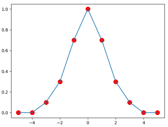
$clipboard_e8e212c015aed62ddb3b2f0a05c1fcf4a.png$

While simplistic, this approximation is likely better than that generated when using the same data points and Newton's method. This is due to the absence of Runge's phenomenon. To make the picture look even better, we can replace the lines by cubic functions. When doing so, we will end up with a number of cubic functions equal to one less than the number of data points - that is, one for every interval between the data points. We call this function $s(x)$ , which can be defined as follows.

$s(x) = \left\{ \begin{array}{lr} s_0(x)=a_0x^3+b_0x^2+c_0x+d_0 & \text{if } x_0\leq x\leq x_1\\ s_1(x)=a_1x^3+b_1x^2+c_1x+d_1 & \text{if } x_1\leq x\leq x_2\\ \vdots\\ s_{n-1}(x)=a_{n-1}x^3+b_{n-1}x^2+c_{n-1}x+d_{n-1} & \text{if } x_{n-1}\leq x\leq x_n\\ \end{array} \right$

Search

Text Color

Text Size

Margin Size

Font Type

THE LAGRANGE POLYNOMIAL

NEWTON INTERPOLATION

3.2.1: Lagrange Polynomial

THE LAGRANGE POLYNOMIAL

3.2.2: Newton interpolation

NEWTON INTERPOLATION

3.2.3: Cubic Splines

Support Center

How can we help?