1.6.4.4: Fractions, counts and ranks- secondary data
- Page ID
- 32626
\( \newcommand{\vecs}[1]{\overset { \scriptstyle \rightharpoonup} {\mathbf{#1}} } \)
\( \newcommand{\vecd}[1]{\overset{-\!-\!\rightharpoonup}{\vphantom{a}\smash {#1}}} \)
\( \newcommand{\dsum}{\displaystyle\sum\limits} \)
\( \newcommand{\dint}{\displaystyle\int\limits} \)
\( \newcommand{\dlim}{\displaystyle\lim\limits} \)
\( \newcommand{\id}{\mathrm{id}}\) \( \newcommand{\Span}{\mathrm{span}}\)
( \newcommand{\kernel}{\mathrm{null}\,}\) \( \newcommand{\range}{\mathrm{range}\,}\)
\( \newcommand{\RealPart}{\mathrm{Re}}\) \( \newcommand{\ImaginaryPart}{\mathrm{Im}}\)
\( \newcommand{\Argument}{\mathrm{Arg}}\) \( \newcommand{\norm}[1]{\| #1 \|}\)
\( \newcommand{\inner}[2]{\langle #1, #2 \rangle}\)
\( \newcommand{\Span}{\mathrm{span}}\)
\( \newcommand{\id}{\mathrm{id}}\)
\( \newcommand{\Span}{\mathrm{span}}\)
\( \newcommand{\kernel}{\mathrm{null}\,}\)
\( \newcommand{\range}{\mathrm{range}\,}\)
\( \newcommand{\RealPart}{\mathrm{Re}}\)
\( \newcommand{\ImaginaryPart}{\mathrm{Im}}\)
\( \newcommand{\Argument}{\mathrm{Arg}}\)
\( \newcommand{\norm}[1]{\| #1 \|}\)
\( \newcommand{\inner}[2]{\langle #1, #2 \rangle}\)
\( \newcommand{\Span}{\mathrm{span}}\) \( \newcommand{\AA}{\unicode[.8,0]{x212B}}\)
\( \newcommand{\vectorA}[1]{\vec{#1}} % arrow\)
\( \newcommand{\vectorAt}[1]{\vec{\text{#1}}} % arrow\)
\( \newcommand{\vectorB}[1]{\overset { \scriptstyle \rightharpoonup} {\mathbf{#1}} } \)
\( \newcommand{\vectorC}[1]{\textbf{#1}} \)
\( \newcommand{\vectorD}[1]{\overrightarrow{#1}} \)
\( \newcommand{\vectorDt}[1]{\overrightarrow{\text{#1}}} \)
\( \newcommand{\vectE}[1]{\overset{-\!-\!\rightharpoonup}{\vphantom{a}\smash{\mathbf {#1}}}} \)
\( \newcommand{\vecs}[1]{\overset { \scriptstyle \rightharpoonup} {\mathbf{#1}} } \)
\( \newcommand{\vecd}[1]{\overset{-\!-\!\rightharpoonup}{\vphantom{a}\smash {#1}}} \)
\(\newcommand{\avec}{\mathbf a}\) \(\newcommand{\bvec}{\mathbf b}\) \(\newcommand{\cvec}{\mathbf c}\) \(\newcommand{\dvec}{\mathbf d}\) \(\newcommand{\dtil}{\widetilde{\mathbf d}}\) \(\newcommand{\evec}{\mathbf e}\) \(\newcommand{\fvec}{\mathbf f}\) \(\newcommand{\nvec}{\mathbf n}\) \(\newcommand{\pvec}{\mathbf p}\) \(\newcommand{\qvec}{\mathbf q}\) \(\newcommand{\svec}{\mathbf s}\) \(\newcommand{\tvec}{\mathbf t}\) \(\newcommand{\uvec}{\mathbf u}\) \(\newcommand{\vvec}{\mathbf v}\) \(\newcommand{\wvec}{\mathbf w}\) \(\newcommand{\xvec}{\mathbf x}\) \(\newcommand{\yvec}{\mathbf y}\) \(\newcommand{\zvec}{\mathbf z}\) \(\newcommand{\rvec}{\mathbf r}\) \(\newcommand{\mvec}{\mathbf m}\) \(\newcommand{\zerovec}{\mathbf 0}\) \(\newcommand{\onevec}{\mathbf 1}\) \(\newcommand{\real}{\mathbb R}\) \(\newcommand{\twovec}[2]{\left[\begin{array}{r}#1 \\ #2 \end{array}\right]}\) \(\newcommand{\ctwovec}[2]{\left[\begin{array}{c}#1 \\ #2 \end{array}\right]}\) \(\newcommand{\threevec}[3]{\left[\begin{array}{r}#1 \\ #2 \\ #3 \end{array}\right]}\) \(\newcommand{\cthreevec}[3]{\left[\begin{array}{c}#1 \\ #2 \\ #3 \end{array}\right]}\) \(\newcommand{\fourvec}[4]{\left[\begin{array}{r}#1 \\ #2 \\ #3 \\ #4 \end{array}\right]}\) \(\newcommand{\cfourvec}[4]{\left[\begin{array}{c}#1 \\ #2 \\ #3 \\ #4 \end{array}\right]}\) \(\newcommand{\fivevec}[5]{\left[\begin{array}{r}#1 \\ #2 \\ #3 \\ #4 \\ #5 \\ \end{array}\right]}\) \(\newcommand{\cfivevec}[5]{\left[\begin{array}{c}#1 \\ #2 \\ #3 \\ #4 \\ #5 \\ \end{array}\right]}\) \(\newcommand{\mattwo}[4]{\left[\begin{array}{rr}#1 \amp #2 \\ #3 \amp #4 \\ \end{array}\right]}\) \(\newcommand{\laspan}[1]{\text{Span}\{#1\}}\) \(\newcommand{\bcal}{\cal B}\) \(\newcommand{\ccal}{\cal C}\) \(\newcommand{\scal}{\cal S}\) \(\newcommand{\wcal}{\cal W}\) \(\newcommand{\ecal}{\cal E}\) \(\newcommand{\coords}[2]{\left\{#1\right\}_{#2}}\) \(\newcommand{\gray}[1]{\color{gray}{#1}}\) \(\newcommand{\lgray}[1]{\color{lightgray}{#1}}\) \(\newcommand{\rank}{\operatorname{rank}}\) \(\newcommand{\row}{\text{Row}}\) \(\newcommand{\col}{\text{Col}}\) \(\renewcommand{\row}{\text{Row}}\) \(\newcommand{\nul}{\text{Nul}}\) \(\newcommand{\var}{\text{Var}}\) \(\newcommand{\corr}{\text{corr}}\) \(\newcommand{\len}[1]{\left|#1\right|}\) \(\newcommand{\bbar}{\overline{\bvec}}\) \(\newcommand{\bhat}{\widehat{\bvec}}\) \(\newcommand{\bperp}{\bvec^\perp}\) \(\newcommand{\xhat}{\widehat{\xvec}}\) \(\newcommand{\vhat}{\widehat{\vvec}}\) \(\newcommand{\uhat}{\widehat{\uvec}}\) \(\newcommand{\what}{\widehat{\wvec}}\) \(\newcommand{\Sighat}{\widehat{\Sigma}}\) \(\newcommand{\lt}{<}\) \(\newcommand{\gt}{>}\) \(\newcommand{\amp}{&}\) \(\definecolor{fillinmathshade}{gray}{0.9}\)These data types arise from modification of the “primary”, original data, mostly from ranked or nominal data that cannot be analyzed head-on. Close to secondary data is an idea of compositional data which are quantitative descriptions of the parts of the whole (probabilities, proportions, percentages etc.)
Percentages, proportions and fractions (ratios) are pretty common and do not need detailed explanation. This is how to calculate percentages (rounded to whole numbers) for our sex data:
Code \(\PageIndex{1}\) (R):
Since it is so easy to lie with proportions, they must be always supplied with the original data. For example, 50% mortality looks extremely high but if it is discovered that there was only 2 patients, then impression is completely different.
Ratios are particularly handy when measured objects have widely varying absolute values. For example, weight is not very useful in medicine while the height-to-weight ratio allows successful diagnostics.
Counts are just numbers of individual elements inside categories. In R, the easiest way to obtain counts is the table() command.
There are many ways to visualize counts and percentages. Bu default, R plots one-dimensional tables (counts) with simple vertical lines (try plot(sex.t) yourself).
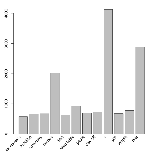
More popular are pie-charts and barplots. However, they represent data badly. There were multiple experiments when people were asked to look on different kinds of plots, and then to report numbers they actually remember. You can run this experiment yourself. Figure \(\PageIndex{1}\) is a barplot of top twelve R commands:
Code \(\PageIndex{2}\) (R):
(We load()’ed binary file to avoid using commands which we did not yet learn; to load binary file from Internet, use load(url(...)). To make bar labels look better, we applied here the “trick” with rotation. Much more simple but less aesthetic solution is barplot(com12, las=2).)
Try looking at this barplot for 3–5 minutes, then withdraw from this book and report numbers seen there, from largest to smallest. Compare with the answer from the end of the chapter.
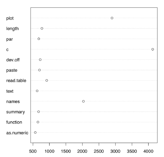
In many experiments like this, researchers found that the most accurately understood graphical feature is the position along the axis, whereas length, angle, area, density and color are each less and less appropriate. This is why from the beginning of R history, pie-charts and barplots were recommended to replace with dotcharts (Figure \(\PageIndex{2}\)):
Code \(\PageIndex{3}\) (R):
We hope you would agree that the dotchart is easier both to understand and to remember. (Of course, it is possible to make this plot even more understandable with sorting like dotchart(rev(sort(com12)))—try it yourself. It is also possible to sort bars, but even sorted barplot is worse then dotchart.)
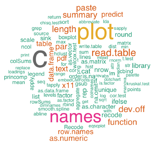
Another useful plot for counts is the word cloud, the image where every item is magnified in accordance with its frequency. This idea came out of text mining tools. To make word clouds in R, one might use the wordcloud package (Figure \(\PageIndex{3}\)):
Code \(\PageIndex{4}\) (R):
 Figure \(\PageIndex{1}\) Barplot of 12 most frequent R commands.
Code \(\PageIndex{5}\) (R):
(New com80 object is a data frame with two columns—check it with str() command. Since wordcloud() “wants” words and frequencies separately, we supplied columns of com80 individually to each argument. To select column, we used square brackets with two arguments: e.g., com80[, 1] is the first column. See more about this in the “Inside R” section.)
Command set.seed() needs more explanation. It freezes random number generator in such a way that immediately after its first use all random numbers are the same on different computers. Word cloud plot uses random numbers, therefore in order to have plots similar between Figure \(\PageIndex{2}\) and your computer, it is better run set.seed()
 Figure \(\PageIndex{2}\) Dotchart, or Cleveland dot plot of 12 most frequent R commands.
immediately before plotting. Its argument should be single integer value, same on all computers. To re-initialize random numbers, run set.seed(NULL).
By the way, NULL object is not just an emptiness, it is a really useful tool. For example, it is easy to remove columns from data frame with command like trees[, 3] <- NULL. If some command “wants” to plot but you do not need this feature, suppress plotting with pdf(file=NULL) command (do not forget to close device with dev.off()).
Compare with your results:
Code \(\PageIndex{6}\) (R):
 Figure \(\PageIndex{3}\) Example of word cloud: 80 important R commands.
Word cloud is a fashionable way to show counts but it has one big minus: whereas it possible to tell which word in more frequent, it is impossible to tell how frequent it is. Dotchart of com80 needs more space (it is better to plot is as big PDF) but there will be both relative and absolute frequencies visible. Try it yourself:
Code \(\PageIndex{7}\) (R):
(We used logarithmic scale to make counts less dispersed and cex parameter to decrease font size.)
While counts and percentages usually come from categorical (nominal) data, ranks usually come from the measurement data, like our heights:
Code \(\PageIndex{8}\) (R):
(The “trick” here was to use names to represent ranks. All R objects, along with values, might bear names.)
Not only integers, but fractions too may serve as rank; the latter happens when there is an even number of equal measurements (i.e., some items are duplicated):
Code \(\PageIndex{9}\) (R):
In general, identical original measurements receive identical ranks. This situation is called a “tie”, just as in sport. Ties may interfere with some nonparametric tests and other calculations based on ranks:
Code \(\PageIndex{10}\) (R):
(If you did not see Rwarnings before, remember that they might appear even if there is nothing wrong. Therefore, ignore them if you do not understand them. However, sometimes warnings bring useful information.)
R always returns a warning if there are ties. It is possible to avoid ties adding small random noise with jitter() command (examples will follow.)
Ranks are widely used in statistics. For example, the popular measure of central tendency, median (see later) is calculated using ranks. They are especially suited for ranked and nonparametric measurement data. Analyses based on ranks are usually more robust but less sensitive.


