1.6.5.2: 1-Dimensional Plots
( \newcommand{\kernel}{\mathrm{null}\,}\)
Our firm has just seven workers. How to analyze the bigger data? Let us first imagine that our hypothetical company prospers and hired one thousand new workers! We add them to our seven data points, with their salaries drawn randomly from interquartile range of the original sample (Figure 1.6.5.2.1):
Code 1.6.5.2.1 (R): Boxplots
In a code above we also see an example of data generation. Function sample() draws values randomly from a distribution or interval. Here we used replace=TRUE, since we needed to pick a lot of values from a much smaller sample. (The argument replace=FALSE might be needed for imitation of a card game, where each card may only be drawn from a deck once.) Please keep in mind that sampling is random and therefore each iteration will give slightly different results.
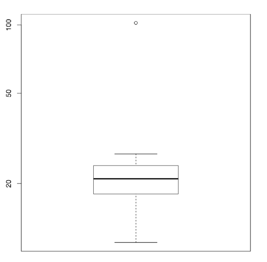 Figure 1.6.5.2.1 The boxplot.
Let us look at the plot. This is the boxplot (“box-and-whiskers” plot). Kathryn’s salary is the highest dot. It is so high, in fact, that we had to add the parameter log="y" to better visualize the rest of the values. The box (main rectangle) itself is bound by second and fourth quartiles, so that its height equals IQR. Thick line in the middle is a median. By default, the “whiskers” extend to the most extreme data point which is no more than 1.5 times the interquartile range from the box. Values that lay farther away are drawn as separate points and are considered outliers. The scheme (Figure 1.6.5.2.2) might help in understanding boxplots.
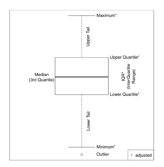 Figure 1.6.5.2.2 The structure of the boxplot (“box-and-whiskers” plot).
Numbers which make the boxplot might be returned with fivenum() command. Boxplot representation was created by a famous American mathematician John W. Tukey as a quick, powerful and consistent way of reflecting main distribution-independent characteristics of the sample. In R, boxplot() is vectorized so we can draw several boxplots at once (Figure 1.6.5.2.3):
Code 1.6.5.2.2 (R): Boxplots
(Parameters of trees were measured in different units, therefore we scale()’d them.)
Histogram is another graphical representation of the sample where range is divided into intervals (bins), and consecutive bars are drawn with their height proportional to the count of values in each bin (Figure 1.6.5.2.4):
Code 1.6.5.2.3 (R): Histograms
(By default, the command hist() would have divided the range into 10 bins, but here we needed 20 and therefore set them manually. Histogram is sometimes a rather cryptic way to display the data. Commands Histp() and Histr() from the asmisc.r will plot histograms together with percentages on the top of each bar, or overlaid with normal curve (or density—see below), respectively. Please try them yourself.)
A numerical analog of a histogram is the function cut():
Code 1.6.5.2.4 (R):
There are other graphical functions, conceptually similar to histograms. The first is stem-and-leaf plot. stem() is a kind of pseudograph, text histogram. Let us see how it treats the original vector salary:
Code 1.6.5.2.5 (R): stem-and-leaf plot
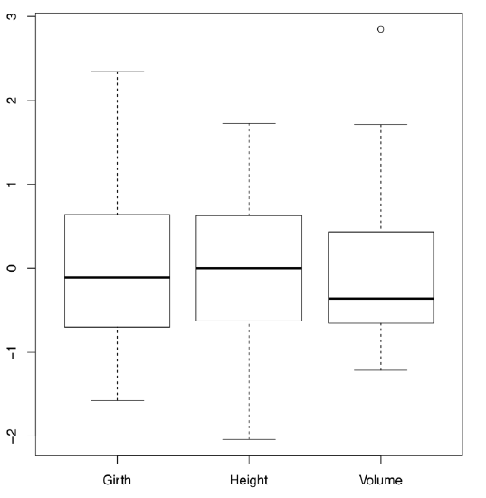 Figure 1.6.5.2.3 Three boxplots, each of them represents one column of the data.
The bar | symbol is a “stem” of the graph. The numbers in front of it are leading digits of the raw values. As you remember, our original data ranged from 11 to 102—therefore we got leading digits from 1 to 10. Each number to the left comes from the next digit of a datum. When we have several values with identical leading digit, like 11 and 19, we place their last digits in a sequence, as “leafs”, to the left of the “stem”. As you see, there are two values between 10 and 20, five values between 20 and 30, etc. Aside from a histogram-like appearance, this function performs an efficient ordering.
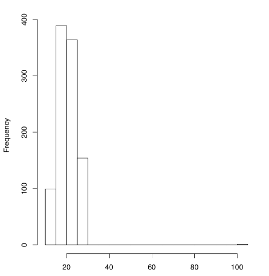 Figure 1.6.5.2.4 Histogram of the 1007 hypothetical employees’ salaries.
Another univariate instrument requires more sophisticated calculations. It is a graph of distribution density, density plot (Figure 1.6.5.2.5):
CodeBox (R) 1.6.5.2.6: Density Plots
Code 1.6.5.2.6 (R): Density Plots
(We used an additional graphic function rug() which supplies an existing plot with a “ruler” which marks areas of highest data density.)
Here the histogram is smoothed, turned into a continuous function. The degree to which it is “rounded” depends on the parameter adjust. Aside from boxplots and a variety of histograms and alike, R and external packages provide many more instruments for univariate plotting.
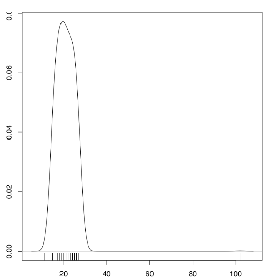 Figure 1.6.5.2.5 Distribution density of the 1007 hypothetical employees’ salaries.
One of simplest is the stripchart. To make stripchart more interesting, we complicated it below using its ability to show individual data points:
Code 1.6.5.2.7 (R): stripchart
(By default, stripchart is horizontal. We used method="jitter" to avoid overplotting, and also scaled all characters to make their distributions comparable. One of stripchart features is that col argument colorizes columns whereas bg argument (which works only for pch from 21 to 25) colorizes rows. We split trees into 3 classes of thickness, and applied these classes as dots background. Note that if data points are shown with multiple colors and/or multiple point types, the legend is always necessary.‘)
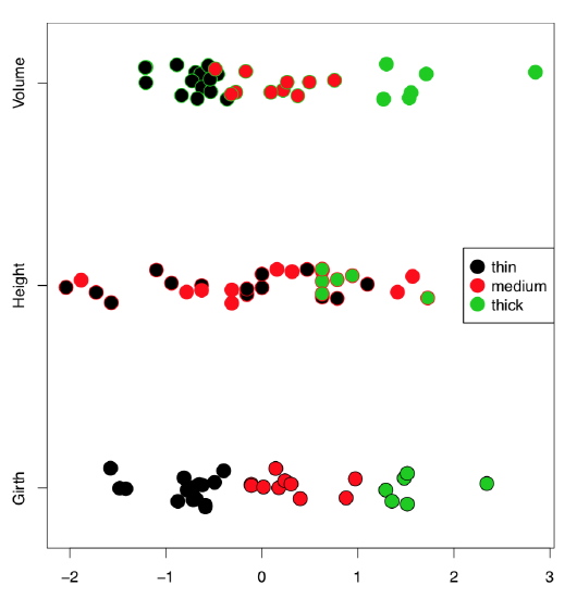 Figure 1.6.5.2.6 Stripchart for modified trees data.
Beeswarm plot requires the external package. It is similar to stripchart but has several advanced methods to disperse points, plus an ability to control the type of individual points (Figure 1.6.5.2.7):
Code 1.6.5.2.8 (R): Beeswarm plots
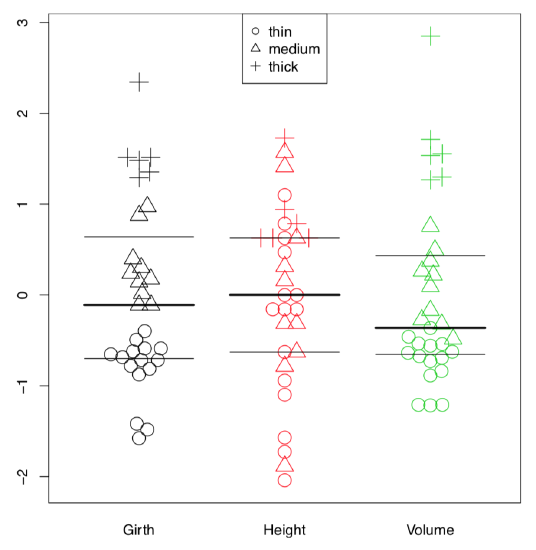 Figure 1.6.5.2.7 Beeswarm plot with boxplot lines.
(Here with bxplot() command we added boxplot lines to a beehive graph in order to visualize quartiles and medians. To overlay, we used an argument add=TRUE.)
And one more useful 1-dimensional plot. It is a similar to both boxplot and density plot (Figure 1.6.5.2.8):
Code 1.6.5.2.1 (R): Bean plots
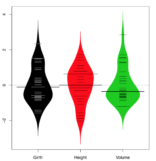 Figure 1.6.5.2.8 Bean plot with overall line and median lines (default lines are means).


