1.6.9.1.3: Plotting...
- Page ID
- 32663
\( \newcommand{\vecs}[1]{\overset { \scriptstyle \rightharpoonup} {\mathbf{#1}} } \)
\( \newcommand{\vecd}[1]{\overset{-\!-\!\rightharpoonup}{\vphantom{a}\smash {#1}}} \)
\( \newcommand{\id}{\mathrm{id}}\) \( \newcommand{\Span}{\mathrm{span}}\)
( \newcommand{\kernel}{\mathrm{null}\,}\) \( \newcommand{\range}{\mathrm{range}\,}\)
\( \newcommand{\RealPart}{\mathrm{Re}}\) \( \newcommand{\ImaginaryPart}{\mathrm{Im}}\)
\( \newcommand{\Argument}{\mathrm{Arg}}\) \( \newcommand{\norm}[1]{\| #1 \|}\)
\( \newcommand{\inner}[2]{\langle #1, #2 \rangle}\)
\( \newcommand{\Span}{\mathrm{span}}\)
\( \newcommand{\id}{\mathrm{id}}\)
\( \newcommand{\Span}{\mathrm{span}}\)
\( \newcommand{\kernel}{\mathrm{null}\,}\)
\( \newcommand{\range}{\mathrm{range}\,}\)
\( \newcommand{\RealPart}{\mathrm{Re}}\)
\( \newcommand{\ImaginaryPart}{\mathrm{Im}}\)
\( \newcommand{\Argument}{\mathrm{Arg}}\)
\( \newcommand{\norm}[1]{\| #1 \|}\)
\( \newcommand{\inner}[2]{\langle #1, #2 \rangle}\)
\( \newcommand{\Span}{\mathrm{span}}\) \( \newcommand{\AA}{\unicode[.8,0]{x212B}}\)
\( \newcommand{\vectorA}[1]{\vec{#1}} % arrow\)
\( \newcommand{\vectorAt}[1]{\vec{\text{#1}}} % arrow\)
\( \newcommand{\vectorB}[1]{\overset { \scriptstyle \rightharpoonup} {\mathbf{#1}} } \)
\( \newcommand{\vectorC}[1]{\textbf{#1}} \)
\( \newcommand{\vectorD}[1]{\overrightarrow{#1}} \)
\( \newcommand{\vectorDt}[1]{\overrightarrow{\text{#1}}} \)
\( \newcommand{\vectE}[1]{\overset{-\!-\!\rightharpoonup}{\vphantom{a}\smash{\mathbf {#1}}}} \)
\( \newcommand{\vecs}[1]{\overset { \scriptstyle \rightharpoonup} {\mathbf{#1}} } \)
\( \newcommand{\vecd}[1]{\overset{-\!-\!\rightharpoonup}{\vphantom{a}\smash {#1}}} \)
\(\newcommand{\avec}{\mathbf a}\) \(\newcommand{\bvec}{\mathbf b}\) \(\newcommand{\cvec}{\mathbf c}\) \(\newcommand{\dvec}{\mathbf d}\) \(\newcommand{\dtil}{\widetilde{\mathbf d}}\) \(\newcommand{\evec}{\mathbf e}\) \(\newcommand{\fvec}{\mathbf f}\) \(\newcommand{\nvec}{\mathbf n}\) \(\newcommand{\pvec}{\mathbf p}\) \(\newcommand{\qvec}{\mathbf q}\) \(\newcommand{\svec}{\mathbf s}\) \(\newcommand{\tvec}{\mathbf t}\) \(\newcommand{\uvec}{\mathbf u}\) \(\newcommand{\vvec}{\mathbf v}\) \(\newcommand{\wvec}{\mathbf w}\) \(\newcommand{\xvec}{\mathbf x}\) \(\newcommand{\yvec}{\mathbf y}\) \(\newcommand{\zvec}{\mathbf z}\) \(\newcommand{\rvec}{\mathbf r}\) \(\newcommand{\mvec}{\mathbf m}\) \(\newcommand{\zerovec}{\mathbf 0}\) \(\newcommand{\onevec}{\mathbf 1}\) \(\newcommand{\real}{\mathbb R}\) \(\newcommand{\twovec}[2]{\left[\begin{array}{r}#1 \\ #2 \end{array}\right]}\) \(\newcommand{\ctwovec}[2]{\left[\begin{array}{c}#1 \\ #2 \end{array}\right]}\) \(\newcommand{\threevec}[3]{\left[\begin{array}{r}#1 \\ #2 \\ #3 \end{array}\right]}\) \(\newcommand{\cthreevec}[3]{\left[\begin{array}{c}#1 \\ #2 \\ #3 \end{array}\right]}\) \(\newcommand{\fourvec}[4]{\left[\begin{array}{r}#1 \\ #2 \\ #3 \\ #4 \end{array}\right]}\) \(\newcommand{\cfourvec}[4]{\left[\begin{array}{c}#1 \\ #2 \\ #3 \\ #4 \end{array}\right]}\) \(\newcommand{\fivevec}[5]{\left[\begin{array}{r}#1 \\ #2 \\ #3 \\ #4 \\ #5 \\ \end{array}\right]}\) \(\newcommand{\cfivevec}[5]{\left[\begin{array}{c}#1 \\ #2 \\ #3 \\ #4 \\ #5 \\ \end{array}\right]}\) \(\newcommand{\mattwo}[4]{\left[\begin{array}{rr}#1 \amp #2 \\ #3 \amp #4 \\ \end{array}\right]}\) \(\newcommand{\laspan}[1]{\text{Span}\{#1\}}\) \(\newcommand{\bcal}{\cal B}\) \(\newcommand{\ccal}{\cal C}\) \(\newcommand{\scal}{\cal S}\) \(\newcommand{\wcal}{\cal W}\) \(\newcommand{\ecal}{\cal E}\) \(\newcommand{\coords}[2]{\left\{#1\right\}_{#2}}\) \(\newcommand{\gray}[1]{\color{gray}{#1}}\) \(\newcommand{\lgray}[1]{\color{lightgray}{#1}}\) \(\newcommand{\rank}{\operatorname{rank}}\) \(\newcommand{\row}{\text{Row}}\) \(\newcommand{\col}{\text{Col}}\) \(\renewcommand{\row}{\text{Row}}\) \(\newcommand{\nul}{\text{Nul}}\) \(\newcommand{\var}{\text{Var}}\) \(\newcommand{\corr}{\text{corr}}\) \(\newcommand{\len}[1]{\left|#1\right|}\) \(\newcommand{\bbar}{\overline{\bvec}}\) \(\newcommand{\bhat}{\widehat{\bvec}}\) \(\newcommand{\bperp}{\bvec^\perp}\) \(\newcommand{\xhat}{\widehat{\xvec}}\) \(\newcommand{\vhat}{\widehat{\vvec}}\) \(\newcommand{\uhat}{\widehat{\uvec}}\) \(\newcommand{\what}{\widehat{\wvec}}\) \(\newcommand{\Sighat}{\widehat{\Sigma}}\) \(\newcommand{\lt}{<}\) \(\newcommand{\gt}{>}\) \(\newcommand{\amp}{&}\) \(\definecolor{fillinmathshade}{gray}{0.9}\)At the beginning, visually check the distribution of data. Make histogram:
Code \(\PageIndex{1}\) (R):
(To see more detailed histogram, increase the number of breaks.)
If for the histogram you want to split data in the specific way (for example, by 20 units, starting from 0 and ending in 100), type:
Code \(\PageIndex{2}\) (R):
Boxplots show outliers, maximum, minimum, quartile range and median for any measurement variable:
Code \(\PageIndex{3}\) (R):
... now for males and females separately, using formula interface:
Code \(\PageIndex{4}\) (R):
There are two commands which together help to check normality of the character:
Code \(\PageIndex{5}\) (R):
(These two separate commands work together to make a single plot, this is why we used semicolon. The more dots on the resulting plot are deviated from the line, the more non-normal is the data.)
Make scatterplot where all bugs represented with small circles. X axis will represent the length whereas Y axis—the weight:
Code \(\PageIndex{6}\) (R):
(type="p" is the default for plot(), therefore it is usually omitted.)
It is possible to change the size of dots varying the cex parameter. Compare
Code \(\PageIndex{7}\) (R):
with
Code \(\PageIndex{8}\) (R):
How to compare? The best way is to have more than one graphical window on the desktop. To start new window, type dev.new().
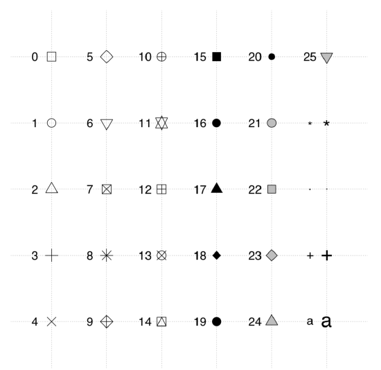
It is also possible to change the type of plotting symbol. Figure \(\PageIndex{1}\) shows their numbers. If you want this table on the computer, you can run:
Code \(\PageIndex{9}\) (R):
 Figure \(\PageIndex{1}\) Point types in R standard plots. For types 21–25, it is possible to specify different background and frame colors.
To obtain similar graphic examples about types of lines, default colors, font faces and plot types, load the gmoon.r\(^{[1]}\)and run:
Code \(\PageIndex{10}\) (R):
Use symbol 2 (empty triangle):
Code \(\PageIndex{11}\) (R):
Use text codes (0/1) for the SEX instead of graphical symbol:
Code \(\PageIndex{12}\) (R):
(Here both commands make one plot together. The first one plots the empty field with axes, the second add there text symbols.)
The same plot is possible to make with the single command, but this works only for one-letter labels:
Code \(\PageIndex{13}\) (R):
If we want these numbers to have different colors, type:
Code \(\PageIndex{14}\) (R):
(Again, both commands make one plot. We added +1 because otherwise female signs would be of 0 color, which is “invisible”.)
Different symbols for males and females:
Code \(\PageIndex{15}\) (R):
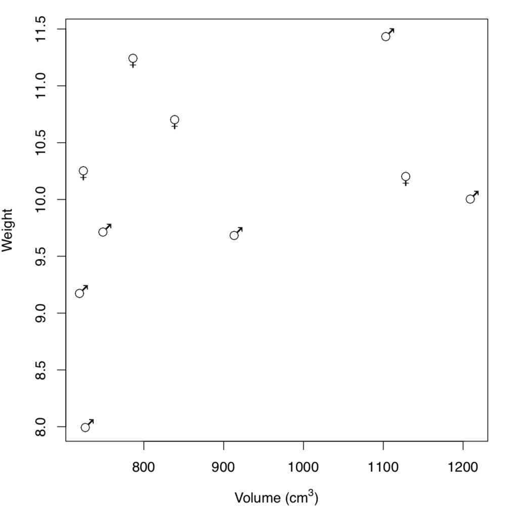
The more complicated variant—use symbols from Hershey fonts\(^{[2]}\) which are internal in R(Figure \(\PageIndex{2}\)):
Code \(\PageIndex{16}\) (R):
(Note also how expression() was employed to make advanced axes labels. Inside expression(), different parts are joined with star *. To know more, run ?plotmath.)
 Figure \(\PageIndex{2}\) Distribution of male and female bugs by size and weight (Hershey fonts used)
We can paint symbols with different colors:
Code \(\PageIndex{17}\) (R):
Finally, it is good to have a legend:
Code \(\PageIndex{18}\) (R):
And then save the plot as PDF file:
Code \(\PageIndex{19}\) (R):
Attention! Saving into the external file, never forget to type dev.off()!
If you do not want any of axis and main labels, insert options main="", xlab="", ylab="" into your plot() command.
There is also a better way to save plots because it does not duplicate to screen and therefore works better in R scripts:
Code \(\PageIndex{20}\) (R):
(Please note here that R issues no warning if the file with the same name is already exist on the disk, it simply erases it and saves the new one. Be careful!)
References
1. With command source("ashipunov.info/r/gmoon.r").
2. To know which symbols are available, run demo(Hershey).


