1.6.9.5: The short R glossary
- Page ID
- 32683
\( \newcommand{\vecs}[1]{\overset { \scriptstyle \rightharpoonup} {\mathbf{#1}} } \)
\( \newcommand{\vecd}[1]{\overset{-\!-\!\rightharpoonup}{\vphantom{a}\smash {#1}}} \)
\( \newcommand{\id}{\mathrm{id}}\) \( \newcommand{\Span}{\mathrm{span}}\)
( \newcommand{\kernel}{\mathrm{null}\,}\) \( \newcommand{\range}{\mathrm{range}\,}\)
\( \newcommand{\RealPart}{\mathrm{Re}}\) \( \newcommand{\ImaginaryPart}{\mathrm{Im}}\)
\( \newcommand{\Argument}{\mathrm{Arg}}\) \( \newcommand{\norm}[1]{\| #1 \|}\)
\( \newcommand{\inner}[2]{\langle #1, #2 \rangle}\)
\( \newcommand{\Span}{\mathrm{span}}\)
\( \newcommand{\id}{\mathrm{id}}\)
\( \newcommand{\Span}{\mathrm{span}}\)
\( \newcommand{\kernel}{\mathrm{null}\,}\)
\( \newcommand{\range}{\mathrm{range}\,}\)
\( \newcommand{\RealPart}{\mathrm{Re}}\)
\( \newcommand{\ImaginaryPart}{\mathrm{Im}}\)
\( \newcommand{\Argument}{\mathrm{Arg}}\)
\( \newcommand{\norm}[1]{\| #1 \|}\)
\( \newcommand{\inner}[2]{\langle #1, #2 \rangle}\)
\( \newcommand{\Span}{\mathrm{span}}\) \( \newcommand{\AA}{\unicode[.8,0]{x212B}}\)
\( \newcommand{\vectorA}[1]{\vec{#1}} % arrow\)
\( \newcommand{\vectorAt}[1]{\vec{\text{#1}}} % arrow\)
\( \newcommand{\vectorB}[1]{\overset { \scriptstyle \rightharpoonup} {\mathbf{#1}} } \)
\( \newcommand{\vectorC}[1]{\textbf{#1}} \)
\( \newcommand{\vectorD}[1]{\overrightarrow{#1}} \)
\( \newcommand{\vectorDt}[1]{\overrightarrow{\text{#1}}} \)
\( \newcommand{\vectE}[1]{\overset{-\!-\!\rightharpoonup}{\vphantom{a}\smash{\mathbf {#1}}}} \)
\( \newcommand{\vecs}[1]{\overset { \scriptstyle \rightharpoonup} {\mathbf{#1}} } \)
\( \newcommand{\vecd}[1]{\overset{-\!-\!\rightharpoonup}{\vphantom{a}\smash {#1}}} \)
\(\newcommand{\avec}{\mathbf a}\) \(\newcommand{\bvec}{\mathbf b}\) \(\newcommand{\cvec}{\mathbf c}\) \(\newcommand{\dvec}{\mathbf d}\) \(\newcommand{\dtil}{\widetilde{\mathbf d}}\) \(\newcommand{\evec}{\mathbf e}\) \(\newcommand{\fvec}{\mathbf f}\) \(\newcommand{\nvec}{\mathbf n}\) \(\newcommand{\pvec}{\mathbf p}\) \(\newcommand{\qvec}{\mathbf q}\) \(\newcommand{\svec}{\mathbf s}\) \(\newcommand{\tvec}{\mathbf t}\) \(\newcommand{\uvec}{\mathbf u}\) \(\newcommand{\vvec}{\mathbf v}\) \(\newcommand{\wvec}{\mathbf w}\) \(\newcommand{\xvec}{\mathbf x}\) \(\newcommand{\yvec}{\mathbf y}\) \(\newcommand{\zvec}{\mathbf z}\) \(\newcommand{\rvec}{\mathbf r}\) \(\newcommand{\mvec}{\mathbf m}\) \(\newcommand{\zerovec}{\mathbf 0}\) \(\newcommand{\onevec}{\mathbf 1}\) \(\newcommand{\real}{\mathbb R}\) \(\newcommand{\twovec}[2]{\left[\begin{array}{r}#1 \\ #2 \end{array}\right]}\) \(\newcommand{\ctwovec}[2]{\left[\begin{array}{c}#1 \\ #2 \end{array}\right]}\) \(\newcommand{\threevec}[3]{\left[\begin{array}{r}#1 \\ #2 \\ #3 \end{array}\right]}\) \(\newcommand{\cthreevec}[3]{\left[\begin{array}{c}#1 \\ #2 \\ #3 \end{array}\right]}\) \(\newcommand{\fourvec}[4]{\left[\begin{array}{r}#1 \\ #2 \\ #3 \\ #4 \end{array}\right]}\) \(\newcommand{\cfourvec}[4]{\left[\begin{array}{c}#1 \\ #2 \\ #3 \\ #4 \end{array}\right]}\) \(\newcommand{\fivevec}[5]{\left[\begin{array}{r}#1 \\ #2 \\ #3 \\ #4 \\ #5 \\ \end{array}\right]}\) \(\newcommand{\cfivevec}[5]{\left[\begin{array}{c}#1 \\ #2 \\ #3 \\ #4 \\ #5 \\ \end{array}\right]}\) \(\newcommand{\mattwo}[4]{\left[\begin{array}{rr}#1 \amp #2 \\ #3 \amp #4 \\ \end{array}\right]}\) \(\newcommand{\laspan}[1]{\text{Span}\{#1\}}\) \(\newcommand{\bcal}{\cal B}\) \(\newcommand{\ccal}{\cal C}\) \(\newcommand{\scal}{\cal S}\) \(\newcommand{\wcal}{\cal W}\) \(\newcommand{\ecal}{\cal E}\) \(\newcommand{\coords}[2]{\left\{#1\right\}_{#2}}\) \(\newcommand{\gray}[1]{\color{gray}{#1}}\) \(\newcommand{\lgray}[1]{\color{lightgray}{#1}}\) \(\newcommand{\rank}{\operatorname{rank}}\) \(\newcommand{\row}{\text{Row}}\) \(\newcommand{\col}{\text{Col}}\) \(\renewcommand{\row}{\text{Row}}\) \(\newcommand{\nul}{\text{Nul}}\) \(\newcommand{\var}{\text{Var}}\) \(\newcommand{\corr}{\text{corr}}\) \(\newcommand{\len}[1]{\left|#1\right|}\) \(\newcommand{\bbar}{\overline{\bvec}}\) \(\newcommand{\bhat}{\widehat{\bvec}}\) \(\newcommand{\bperp}{\bvec^\perp}\) \(\newcommand{\xhat}{\widehat{\xvec}}\) \(\newcommand{\vhat}{\widehat{\vvec}}\) \(\newcommand{\uhat}{\widehat{\uvec}}\) \(\newcommand{\what}{\widehat{\wvec}}\) \(\newcommand{\Sighat}{\widehat{\Sigma}}\) \(\newcommand{\lt}{<}\) \(\newcommand{\gt}{>}\) \(\newcommand{\amp}{&}\) \(\definecolor{fillinmathshade}{gray}{0.9}\)The short R glossary
This very short glossary will help to find the corresponding R command for the most widespread statistical terms. This is similar to the “reverse index” which might be useful when you know what to do but do not know which R command to use.
Akaike’s Information Criterion, AIC – AIC() – criterion of the model optimality; the best model usually corresponds with minimal AIC.
analysis of variance, ANOVA – aov() – the family of parametric tests, used to compare multiple samples.
analysis of covariance, ANCOVA – lm(response ~ influence*factor) – just another variant of linear models, compares several regression lines.
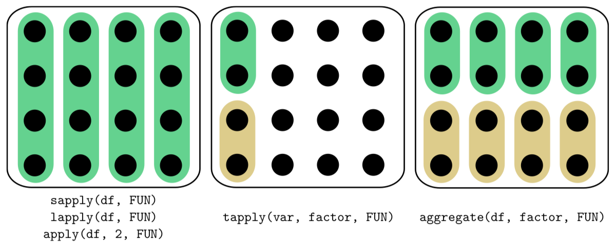
“apply family” – aggregate(), apply(), lapply(), sapply(), tapply() and others — R functions which help to avoid loops, repeats of the same sequence of commands. Differences between most frequently used functions from this family (applied on data frame) are shown on Figure \(\PageIndex{1}\).

arithmetic mean, mean, average – mean() – sum of all sample values divides to their number.
bar plot – barplot() – the diagram to represent several numeric values (e.g., counts).
Bartlett test – bartlett.test() – checks the null if variances of samples are equal (ANOVA assumption).
bootstrap – sample() and many others – technique of sample sub-sampling to estimate population statistics.
boxplot – boxplot() – the diagram to represent main features of one or several samples.
Chi-squared test – chisq.test() – helps to check if there is a association between rows and columns in the contingency table.
cluster analisys, hierarchical – hclust() – visualization of objects’ dissimilarities as dendrogram (tree).
confidence interval – the range where some population value (mean, median etc.) might be located with given probability.
correlation analysis – cor.test() – group of methods which allow to describe the determination between several samples.
correlation matrix – cor() – returns correlation coefficients for all pairs of samples.
data types – there is a list (with synonyms):
-
measurement:
-
continuous;
-
meristic, discrete, discontinuous;
-
-
ranked, ordinal;
-
categorical, nominal.
distance matrix – dist(), daisy(), vegdist() – calculates distance (dissimilarity) between objects.
distribution – the “layout”, the “shape” of data; theoretical distribution shows how data should look whereas sample distribution shows how data looks in reality.
F-test – var.test() – parametric test used to compare variations in two samples.
Fisher’s exact test – fisher.test() – similar to chi-squared but calculates (not estimates) p-value; recommended for small data.
generalized linear models – glm() – extension of linear models allowing (for example) the binary response; the latter is the logistic regression.
histogram – hist() – diagram to show frequencies of different values in the sample.
interquartile range – IQR() – the distance between second and fourth quartile, the robust method to show variability.
Kolmogorov-Smirnov test – ks.test() – used to compare two distributions, including comparison between sample distribution and normal distribution.
Kruskal-Wallis test – kruskal.test() – used to compare multiple samples, this is nonparametric replacement of ANOVA.
linear discriminant analysis – lda() – multivariate method, allows to create classification based on the training sample.
linear regression – lm() – researches linear relationship (linear regression) between objects.
long form – stack(); unstack() – the variant of data representation where group (feature) IDs and data are both vertical, in columns:
SEX SIZE
M 1
M 1
F 2
F 1
LOESS – loess.smooth() – Locally wEighted Scatterplot Smoothing.
McNemar’s test – mcnemar.test() – similar to chi-squared but allows to check association in case of paired observations.
Mann-Whitney test – wilcox.test() – see the Wilcoxon test.
median – median() – the value splitting sample in two halves.
model formulas – formula() – the way to describe the statistical model briefly:
-
response ~ influence: analysis of the regression;
-
response ~ influence1 + influence2: analysis of multiple regression, additive model;
-
response ~ factor: one-factor ANOVA;
-
response ~ factor1 + factor2: multi-factor ANOVA;
-
response ~ influence * factor: analysis of covariation, model with interactions, expands into “response ~ influence + influence : factor”.
Operators used in formulas:
-
all predictors (influences and factors) from the previous model (used together with update());
-
adds factor or influence;
-
removes factor or influence;
-
interaction;
-
all logical combinations of factors and influences;
-
inclusion, “factor1 / factor2” means that factor2 is embedded in factor1 (like street is “embedded” in district, and district in city);
-
condition, “factor1 | factor2” means “split factor1 by the levels of factor2”;
-
intercept, so response ~ influence - 1 means linear model without intercept;
-
returns arithmetical values for everything in parentheses. It is also used in data.frame() command to skip conversion into factor for character columns.
-
multidimensional scaling, MDS – cmdscale() – builds something like a map from the distance matrix.
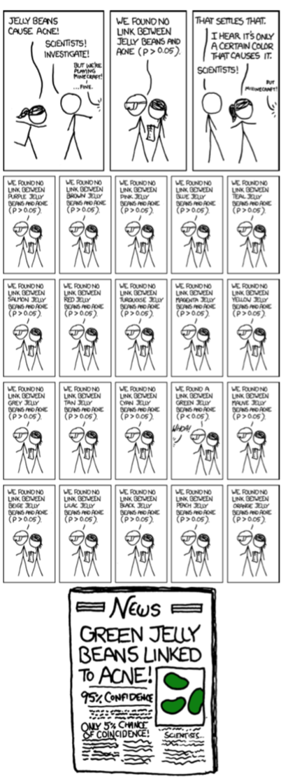
multiple comparisons – p.adjust() – see XKCD comic for the best explanation (Figure \(\PageIndex{2}\)).
nonparametric – not related with a specific theoretical distribution, useful for the analysis of arbitrary data.
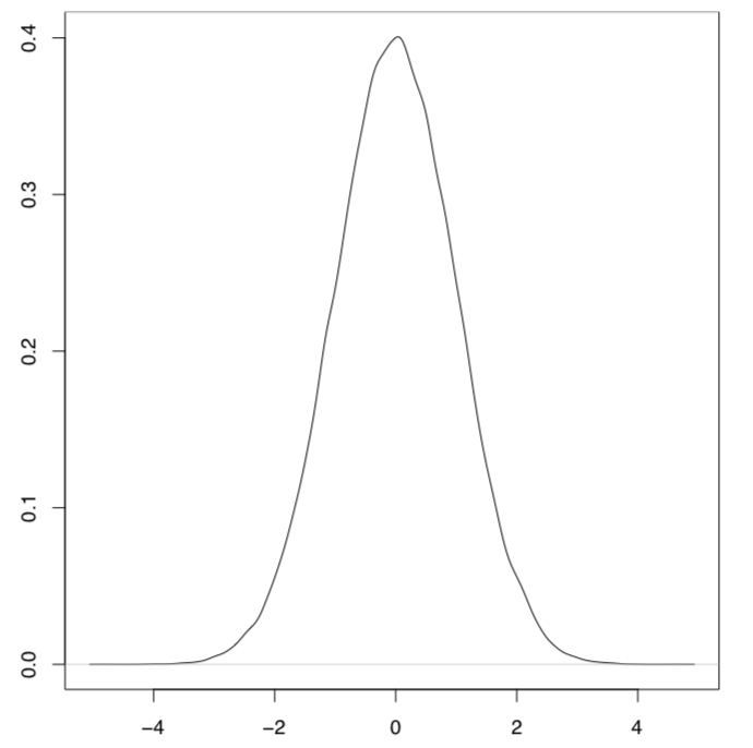
normal distribution plot – plot(density(rnorm(1000000))) – “bell”, “hat” (Figure \(\PageIndex{3}\)).
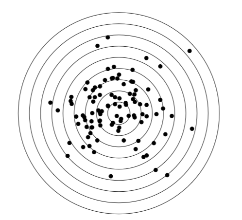
normal distribution – rnorm() – the most important theoretical distribution, the basement of parametric methods; appears, for example if one will shot into the target for a long time and then measure all distances to the center (Figure \(\PageIndex{4}\)):

Code \(\PageIndex{1}\) (Python):
library(plotrix)
plot(c(-1, 1), c(-1, 1), type="n", xlab="", ylab="", axes=FALSE)
for(n in seq(0.1, 0.9, 0.1)) draw.circle(0, 0, n)
set.seed(11); x <- rnorm(100, sd=.28); y <- rnorm(100, sd=.28)
points(x, y, pch=19)

one-way test – oneway.test() – similar to simple ANOVA but omits the homogeneity of variances assumption.
pairwise t-test – pairwise.t.test() – parametric post hoc test with adjustment for multiple comparisons.
pairwise Wilcoxon test – pairwise.wilcox.test() – nonparametric post hoc test with adjustment for multiple comparisons.
parametric – corresponding with the known (in this book: normal, see) distribution, suitable to the analysis of the normally distributed data.

post hoc – tests which check all groups pairwise; contrary to the name, it is not necessary to run them after something else.
principal component analysis – princomp(), prcomp() – multivariate method “projected” multivariate cloud onto the plane of principal components.
proportion test – prop.test() – checks if proportions are equal.
p-value – probability to obtain the estimated value if the null hypothesis is true; if p-value is below the threshold then null hypothesis should be rejected (see the “two-dimensional data” chapter for the explanation about statistical hypotheses).
robust – not so sensitive to outliers, many robust methods are also nonparametric.
quantile – quantile() – returns values of quantiles (by default, values which cut off 0, 25, 50, 75 and 100% of the sample).
scatterplot – plot(x, y) – plot showing the correspondence between two variables.
Shapiro-Wilk test – shapiro.test() – test for checking the normality of the sample.
short form – stack(); unstack() – the variant of data representation where group IDs are horizontal (they are columns):
M.SIZE F.SIZE
1 2
1 1
standard deviation – sd() – square root of the variance.
standard error, SE – sd(x)/sqrt(length(x)) – normalized variance.
stem-and-leaf plot – stem() – textual plot showing frequencies of values in the sample, alternative for histogram.
t-test – t.test() – the family of parametric tests which are used to estimate and/or compare mean values from one or two samples.
Tukey HSD – TukeyHSD() – parametric post hoc test for multiple comparisons which calculates Tukey Honest Significant Differences (confidence intervals).
Tukey’s line – line() – linear relation fit robustly, with medians of subgroups.
uniform distribution – runif() – distribution where every value has the same probability.
variance – var() – the averaged difference between mean and all other sample values.
Wilcoxon test – wilcox.test() – used to estimate and/or compare medians from one or two samples, this is the nonparametric replacement of the t-test.


