
1.4: Graphs of Equations with Two Variables
- Page ID
- 35471
\( \newcommand{\vecs}[1]{\overset { \scriptstyle \rightharpoonup} {\mathbf{#1}} } \)
\( \newcommand{\vecd}[1]{\overset{-\!-\!\rightharpoonup}{\vphantom{a}\smash {#1}}} \)
\( \newcommand{\dsum}{\displaystyle\sum\limits} \)
\( \newcommand{\dint}{\displaystyle\int\limits} \)
\( \newcommand{\dlim}{\displaystyle\lim\limits} \)
\( \newcommand{\id}{\mathrm{id}}\) \( \newcommand{\Span}{\mathrm{span}}\)
( \newcommand{\kernel}{\mathrm{null}\,}\) \( \newcommand{\range}{\mathrm{range}\,}\)
\( \newcommand{\RealPart}{\mathrm{Re}}\) \( \newcommand{\ImaginaryPart}{\mathrm{Im}}\)
\( \newcommand{\Argument}{\mathrm{Arg}}\) \( \newcommand{\norm}[1]{\| #1 \|}\)
\( \newcommand{\inner}[2]{\langle #1, #2 \rangle}\)
\( \newcommand{\Span}{\mathrm{span}}\)
\( \newcommand{\id}{\mathrm{id}}\)
\( \newcommand{\Span}{\mathrm{span}}\)
\( \newcommand{\kernel}{\mathrm{null}\,}\)
\( \newcommand{\range}{\mathrm{range}\,}\)
\( \newcommand{\RealPart}{\mathrm{Re}}\)
\( \newcommand{\ImaginaryPart}{\mathrm{Im}}\)
\( \newcommand{\Argument}{\mathrm{Arg}}\)
\( \newcommand{\norm}[1]{\| #1 \|}\)
\( \newcommand{\inner}[2]{\langle #1, #2 \rangle}\)
\( \newcommand{\Span}{\mathrm{span}}\) \( \newcommand{\AA}{\unicode[.8,0]{x212B}}\)
\( \newcommand{\vectorA}[1]{\vec{#1}} % arrow\)
\( \newcommand{\vectorAt}[1]{\vec{\text{#1}}} % arrow\)
\( \newcommand{\vectorB}[1]{\overset { \scriptstyle \rightharpoonup} {\mathbf{#1}} } \)
\( \newcommand{\vectorC}[1]{\textbf{#1}} \)
\( \newcommand{\vectorD}[1]{\overrightarrow{#1}} \)
\( \newcommand{\vectorDt}[1]{\overrightarrow{\text{#1}}} \)
\( \newcommand{\vectE}[1]{\overset{-\!-\!\rightharpoonup}{\vphantom{a}\smash{\mathbf {#1}}}} \)
\( \newcommand{\vecs}[1]{\overset { \scriptstyle \rightharpoonup} {\mathbf{#1}} } \)
\(\newcommand{\longvect}{\overrightarrow}\)
\( \newcommand{\vecd}[1]{\overset{-\!-\!\rightharpoonup}{\vphantom{a}\smash {#1}}} \)
\(\newcommand{\avec}{\mathbf a}\) \(\newcommand{\bvec}{\mathbf b}\) \(\newcommand{\cvec}{\mathbf c}\) \(\newcommand{\dvec}{\mathbf d}\) \(\newcommand{\dtil}{\widetilde{\mathbf d}}\) \(\newcommand{\evec}{\mathbf e}\) \(\newcommand{\fvec}{\mathbf f}\) \(\newcommand{\nvec}{\mathbf n}\) \(\newcommand{\pvec}{\mathbf p}\) \(\newcommand{\qvec}{\mathbf q}\) \(\newcommand{\svec}{\mathbf s}\) \(\newcommand{\tvec}{\mathbf t}\) \(\newcommand{\uvec}{\mathbf u}\) \(\newcommand{\vvec}{\mathbf v}\) \(\newcommand{\wvec}{\mathbf w}\) \(\newcommand{\xvec}{\mathbf x}\) \(\newcommand{\yvec}{\mathbf y}\) \(\newcommand{\zvec}{\mathbf z}\) \(\newcommand{\rvec}{\mathbf r}\) \(\newcommand{\mvec}{\mathbf m}\) \(\newcommand{\zerovec}{\mathbf 0}\) \(\newcommand{\onevec}{\mathbf 1}\) \(\newcommand{\real}{\mathbb R}\) \(\newcommand{\twovec}[2]{\left[\begin{array}{r}#1 \\ #2 \end{array}\right]}\) \(\newcommand{\ctwovec}[2]{\left[\begin{array}{c}#1 \\ #2 \end{array}\right]}\) \(\newcommand{\threevec}[3]{\left[\begin{array}{r}#1 \\ #2 \\ #3 \end{array}\right]}\) \(\newcommand{\cthreevec}[3]{\left[\begin{array}{c}#1 \\ #2 \\ #3 \end{array}\right]}\) \(\newcommand{\fourvec}[4]{\left[\begin{array}{r}#1 \\ #2 \\ #3 \\ #4 \end{array}\right]}\) \(\newcommand{\cfourvec}[4]{\left[\begin{array}{c}#1 \\ #2 \\ #3 \\ #4 \end{array}\right]}\) \(\newcommand{\fivevec}[5]{\left[\begin{array}{r}#1 \\ #2 \\ #3 \\ #4 \\ #5 \\ \end{array}\right]}\) \(\newcommand{\cfivevec}[5]{\left[\begin{array}{c}#1 \\ #2 \\ #3 \\ #4 \\ #5 \\ \end{array}\right]}\) \(\newcommand{\mattwo}[4]{\left[\begin{array}{rr}#1 \amp #2 \\ #3 \amp #4 \\ \end{array}\right]}\) \(\newcommand{\laspan}[1]{\text{Span}\{#1\}}\) \(\newcommand{\bcal}{\cal B}\) \(\newcommand{\ccal}{\cal C}\) \(\newcommand{\scal}{\cal S}\) \(\newcommand{\wcal}{\cal W}\) \(\newcommand{\ecal}{\cal E}\) \(\newcommand{\coords}[2]{\left\{#1\right\}_{#2}}\) \(\newcommand{\gray}[1]{\color{gray}{#1}}\) \(\newcommand{\lgray}[1]{\color{lightgray}{#1}}\) \(\newcommand{\rank}{\operatorname{rank}}\) \(\newcommand{\row}{\text{Row}}\) \(\newcommand{\col}{\text{Col}}\) \(\renewcommand{\row}{\text{Row}}\) \(\newcommand{\nul}{\text{Nul}}\) \(\newcommand{\var}{\text{Var}}\) \(\newcommand{\corr}{\text{corr}}\) \(\newcommand{\len}[1]{\left|#1\right|}\) \(\newcommand{\bbar}{\overline{\bvec}}\) \(\newcommand{\bhat}{\widehat{\bvec}}\) \(\newcommand{\bperp}{\bvec^\perp}\) \(\newcommand{\xhat}{\widehat{\xvec}}\) \(\newcommand{\vhat}{\widehat{\vvec}}\) \(\newcommand{\uhat}{\widehat{\uvec}}\) \(\newcommand{\what}{\widehat{\wvec}}\) \(\newcommand{\Sighat}{\widehat{\Sigma}}\) \(\newcommand{\lt}{<}\) \(\newcommand{\gt}{>}\) \(\newcommand{\amp}{&}\) \(\definecolor{fillinmathshade}{gray}{0.9}\)Plot Points on a Rectangular Coordinate System
Just like maps use a grid system to identify locations, a grid system is used in algebra to show a relationship between two variables in a rectangular coordinate system. The rectangular coordinate system is also called the xy-plane or the “Cartesian coordinate plane” (after the French mathematician Rene Descartes).
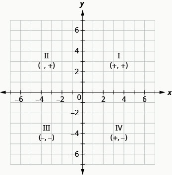
The rectangular coordinate system is formed by two intersecting number lines, one horizontal and one vertical. The horizontal number line is called the \(x\)-axis. The vertical number line is called the \(y\)-axis. These axes divide a plane into four regions, called quadrants. The quadrants are identified by Roman numerals, beginning on the upper right and proceeding counterclockwise. See Figure \(\PageIndex{1}\). Any point in the plane can be located by indicating a position on the horizontal number line and a position on the vertical number line.

In the rectangular coordinate system, every point is represented by an ordered pair. The first number in the ordered pair is the \(x\)-coordinate of the point, representing its horizontal position, and the second number is the \(y\)-coordinate of the point, representing its vertical position. The phrase “ordered pair” means that the order is important.
ORDERED PAIR
An ordered pair \((x,y)\) gives the coordinates of a point in a rectangular coordinate system. The first number is the \(x\)-coordinate. The second number is the \(y\)-coordinate.

What is the ordered pair of the point where the axes cross? At that point both coordinates are zero, so its ordered pair is \((0,0)\).The point \((0,0)\) has a special name. It is called the origin.
THE ORIGIN
The point \((0,0)\) is called the origin. It is the point where the \(x\)-axis and \(y\)-axis intersect.
We use the coordinates to locate a point on the xy-plane. Let’s plot the point \((1,3)\) as an example. First, locate 1 on the x-axis and lightly sketch a vertical line through \(x=1\). Then, locate 3 on the y-axis and sketch a horizontal line through y=3.y=3. Now, find the point where these two lines meet—that is the point with coordinates \((1,3)\). See Figure.
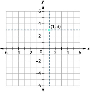
Notice that the vertical line through \(x=1\) and the horizontal line through \(y=3\) are not part of the graph. We just used them to help us locate the point \((1,3)\).
When one of the coordinate is zero, the point lies on one of the axes. In Figure the point \((0,4)\) is on the y-axis and the point \((−2,0)\) is on the x-axis.
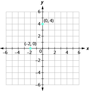
Figure \(\PageIndex{3}\)
POINTS ON THE AXES
Points with a y-coordinate equal to 0 are on the x-axis, and have coordinates \((a,0)\).
Points with an x-coordinate equal to 0 are on the y-axis, and have coordinates \((0,b)\).
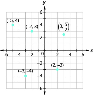
Example \(\PageIndex{1}\)
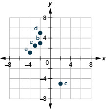
Plot each point in the rectangular coordinate system and identify the quadrant in which the point is located:
ⓐ \((−5,4\)) ⓑ \((−3,−4)\) ⓒ \((2,−3)\) ⓓ \((0,−1)\) ⓔ \((3,\dfrac{5}{2})\).
- Answer
-
The first number of the coordinate pair is the x-coordinate, and the second number is the y-coordinate. To plot each point, sketch a vertical line through the x-coordinate and a horizontal line through the y-coordinate. Their intersection is the point.
ⓐ Since \(x=−5\), the point is to the left of the y-axis. Also, since \(y=4\), the point is above the x-axis. The point \((−5,4)\) is in Quadrant II.
ⓑ Since \(x=−3\), the point is to the left of the y-axis. Also, since \(y=−4\), the point is below the x-axis. The point \((−3,−4)\) is in Quadrant III.
ⓒ Since \(x=2\), the point is to the right of the y-axis. Since \(y=−3\), the point is below the x-axis. The point \((2,−3)\) is in Quadrant IV.
ⓓ Since \(x=0\), the point whose coordinates are \((0,−1)\) is on the y-axis.
ⓔ Since \(x=3\), the point is to the right of the y-axis. Since \(y=\dfrac{5}{2})\), the point is above the x-axis. (It may be helpful to write \(\dfrac{5}{2})\) as a mixed number or decimal.) The point \((3,\dfrac{5}{2})\) is in Quadrant I.
Example \(\PageIndex{2}\)
Plot each point in a rectangular coordinate system and identify the quadrant in which the point is located:
ⓐ \((−2,1)\) ⓑ \((−3,−1)\) ⓒ \((4,−4)\) ⓓ \((−4,4)\) ⓔ \((−4,\dfrac{3}{2})\)
- Answer
-
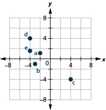
Example \(\PageIndex{3}\)
Plot each point in a rectangular coordinate system and identify the quadrant in which the point is located:
ⓐ \((−4,1)\) ⓑ \((−2,3)\) ⓒ \((2,−5)\) ⓓ \((−2,5)\) ⓔ \((−3,\dfrac{5}{2})\)
- Answer
-
The signs of the x-coordinate and y-coordinate affect the location of the points. You may have noticed some patterns as you graphed the points in the previous example. We can summarize sign patterns of the quadrants in this way:
QUADRANTS
| Quadrant I | Quadrant II | Quadrant III | Quadrant IV |
| \((x,y)\) | \((x,y)\) | \((x,y)\) | \((x,y)\) |
| \((+,+)\) | \((−,+)\) | \((−,−)\) | \((+,−)\) |
Solution Set for an Equation with Two Variables
Equations with two variables (often the variables are names \(x\) and \(y\)) usually have infinitely many solutions. For every number that is substituted for one variable \(x\) we can look for corresponding \(y\)-values that make the equation true. If we find one, this pair of values is a solution to the equation and it can be represented by the ordered pair \((x,y)\). When we substitute these values of x and y into the equation, the result is a true statement, because the value on the left side is equal to the value on the right side.
SOLUTION OF A LINEAR EQUATION IN TWO VARIABLES
An ordered pair \((x,y)\) is a solution of an equation if the equation is a true statement when the \(x\)- and \(y\)-values of the ordered pair are substituted into the equation.
The solution set for an equation with two variables is the set of all ordered pairs that make the equation true. We can plot solutions in the rectangular coordinate system. A graph of an equation is a visual representation of all the solutions of the equation. It is an example of the saying, “A picture is worth a thousand words.” Every point on the graph is a solution of the equation. And, every solution of this equation is on the graph. Points not on the graph are not solutions!
GRAPH OF An EQUATION
The graph of an equation in two variables is the set of all ordered pair solutions to that equation, plotted in the rectangular coordinate system.
- Every point on the graph is a solution of the equation.
- Every solution of this equation is a point on this graph.