4.3: Graphing Functions

Learning Objectives

• Use concavity and inflection points to explain how the sign of the second derivative affects the shape of a function’s graph.
• Explain the concavity test for a function over an open interval.
• Explain the relationship between a function and its first and second derivatives.
• State the second derivative test for local extrema.

In this section, we see how the first and second derivatives provide information about the extrema and shape of a graph by describing whether the graph of a function curves upward or curves downward. Now that we have developed the tools we need to determine where a function is increasing and decreasing, as well as acquired an understanding of the basic shape of the graph, we can provide accurate graphs of a large variety of functions.

Guidelines for Drawing the Graph of a Function

We now have enough analytical tools to draw graphs of a wide variety of algebraic and transcendental functions. Before showing how to graph specific functions, let’s look at a general strategy to use when graphing any function.

Problem-Solving Strategy: Drawing the Graph of a Function

Given a function \(f\), use the following steps to sketch a graph of \(f\):

1. Determine the domain of the function.
2. Locate the \(x\)- and \(y\)-intercepts.
3. Evaluate \(\displaystyle \lim_{x→∞}f(x)\) and \(\displaystyle \lim_{x→−∞}f(x)\) to determine the end behavior. If either of these limits is a finite number \(L\), then \(y=L\) is a horizontal asymptote. If either of these limits is \(∞\) or \(−∞\), determine whether \(f\) has an oblique asymptote. If \(i\)s a rational function such that \(f(x)=\dfrac{p(x)}{q(x)}\), where the degree of the numerator is greater than the degree of the denominator, then \(f\) can be written as \[f(x)=\frac{p(x)}{q(x)}=g(x)+\frac{r(x)}{q(x),}\] where the degree of \(r(x)\) is less than the degree of \(q(x)\). The values of \(f(x)\) approach the values of \(g(x)\) as \(x→±∞\). If \(g(x)\) is a linear function, it is known as an oblique asymptote.
4. Determine whether \(f\) has any vertical asymptotes.
5. Calculate \(f′.\) Find all critical points and determine the intervals where \(f\) is increasing and where \(f\) is decreasing. Determine whether \(f\) has any local extrema.
6. Calculate \(f''.\) Determine the intervals where \(f\) is concave up and where \(f\) is concave down. Use this information to determine whether \(f\) has any inflection points. The second derivative can also be used as an alternate means to determine or verify that \(f\) has a local extremum at a critical point.

Now let’s use this strategy to graph several different functions. We start by graphing a polynomial function.

Example \(\PageIndex{1}\): Sketching a Graph of a Polynomial

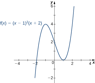
Sketch a graph of \(f(x)=(x−1)^2(x+2).\)

Solution

Step 1: Since \(f\) is a polynomial, the domain is the set of all real numbers.

Step 2: When \(x=0,\; f(x)=2.\) Therefore, the \(y\)-intercept is \((0,2)\). To find the \(x\)-intercepts, we need to solve the equation \((x−1)^2(x+2)=0\), gives us the \(x\)-intercepts \((1,0)\) and \((−2,0)\)

Step 3: We need to evaluate the end behavior of \(f.\) As \(x→∞, \;(x−1)^2→∞\) and \((x+2)→∞\). Therefore, \(\displaystyle \lim_{x→∞}f(x)=∞\).

As \(x→−∞, \;(x−1)^2→∞\) and \((x+2)→−∞\). Therefore, \(\displaystyle \lim_{x→∞}f(x)=−∞\).

To get even more information about the end behavior of \(f\), we can multiply the factors of \(f\). When doing so, we see that

\[f(x)=(x−1)^2(x+2)=x^3−3x+2. \nonumber\]

Since the leading term of \(f\) is \(x^3\), we conclude that \(f\) behaves like \(y=x^3\) as \(x→±∞.\)

Step 4: Since \(f\) is a polynomial function, it does not have any vertical asymptotes.

Step 5: The first derivative of \(f\) is

\[f′(x)=3x^2−3. \nonumber\]

Therefore, \(f\) has two critical points: \(x=1,−1.\) Divide the interval \((−∞,∞)\) into the three smaller intervals: \((−∞,−1), \;(−1,1)\), and \((1,∞)\). Then, choose test points \(x=−2, x=0\), and \(x=2\) from these intervals and evaluate the sign of \(f′(x)\) at each of these test points, as shown in the following table.

Interval	Test point	Sign of Derivative \(f'(x)=3x^2−3=3(x−1)(x+1)\)	Conclusion
\((−∞,−1)\)	\(x=−2\)	\((+)(−)(−)=+\)	\(f\) is increasing
\((−1,1)\)	\(x=0\)	\((+)(−)(+)=−\)	\(f\) decreasing
\((1,∞)\)	\(x=2\)	\((+)(+)(+)=+\)	\(f\) is increasing

From the table, we see that \(f\) has a local maximum at \(x=−1\) and a local minimum at \(x=1\). Evaluating \(f(x)\) at those two points, we find that the local maximum value is \(f(−1)=4\) and the local minimum value is \(f(1)=0.\)

Step 6: The second derivative of \(f\) is

\[f''(x)=6x. \nonumber\]

The second derivative is zero at \(x=0.\) Therefore, to determine the concavity of \(f\), divide the interval \((−∞,∞)\) into the smaller intervals \((−∞,0)\) and \((0,∞)\), and choose test points \(x=−1\) and \(x=1\) to determine the concavity of \(f\) on each of these smaller intervals as shown in the following table.

Interval	Test Point	Sign of \(''(x)=6x\)	Conclusion
\((−∞,0)\)	\(x=−1\)	\(−\)	\(f\) is concave down..
\((0,∞)\)	\(x=1\)	\(+\)	\(f\) is concave up.

We note that the information in the preceding table confirms the fact, found in step \(5\), that f has a local maximum at \(x=−1\) and a local minimum at \(x=1\). In addition, the information found in step \(5\)—namely, \(f\) has a local maximum at \(x=−1\) and a local minimum at \(x=1\), and \(f′(x)=0\) at those points—combined with the fact that \(f''\) changes sign only at \(x=0\) confirms the results found in step \(6\) on the concavity of \(f\).

Combining this information, we arrive at the graph of \(f(x)=(x−1)^2(x+2)\) shown in the following graph.

Exercise \(\PageIndex{1}\)

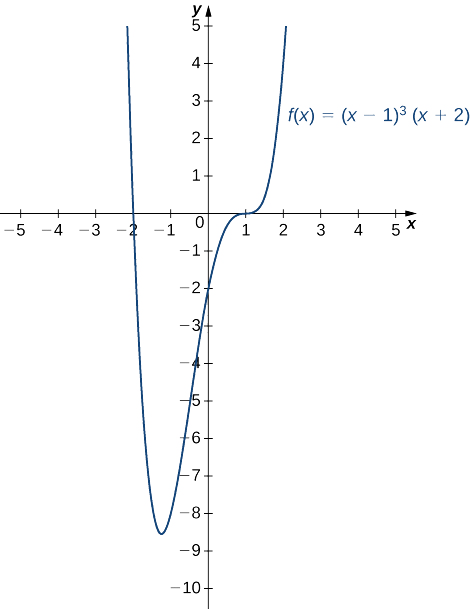
Sketch a graph of \(f(x)=(x−1)^3(x+2).\)

Hint

\(f\) is a fourth-degree polynomial.

Answer

Example \(\PageIndex{2}\): Sketching a Rational Function

Sketch the graph of \(f(x)=\dfrac{x^2}{1−x^2}\).

Solution

Step 1: The function \(f\) is defined as long as the denominator is not zero. Therefore, the domain is the set of all real numbers \(x\) except \(x=±1.\)

Step 2: Find the intercepts. If \(x=0,\) then \(f(x)=0\), so \(0\) is an intercept. If \(y=0\), then \(\dfrac{x^2}{1−x^2}=0,\) which implies \(x=0\). Therefore, \((0,0)\) is the only intercept.

Step 3: Evaluate the limits at infinity. Since \(f\)is a rational function, divide the numerator and denominator by the highest power in the denominator: \(x^2\).We obtain

\(\displaystyle \lim_{x→±∞}\frac{x^2}{1−x^2}=\lim_{x→±∞}\frac{1}{\frac{1}{x^2}−1}=−1.\)

Therefore, \(f\) has a horizontal asymptote of \(y=−1\) as \(x→∞\) and \(x→−∞.\)

Step 4: To determine whether \(f\) has any vertical asymptotes, first check to see whether the denominator has any zeroes. We find the denominator is zero when \(x=±1\). To determine whether the lines \(x=1\) or \(x=−1\) are vertical asymptotes of \(f\), evaluate \(\displaystyle \lim_{x→1}f(x)\) and \(\displaystyle \lim_{x→−1}f(x)\). By looking at each one-sided limit as \(x→1,\) we see that

\(\displaystyle \lim_{x→1^+}\frac{x^2}{1−x^2}=−∞\) and \(\displaystyle \lim_{x→1^−}\frac{x^2}{1−x^2}=∞.\)

In addition, by looking at each one-sided limit as \(x→−1,\) we find that

\(\displaystyle \lim_{x→−1^+}\frac{x^2}{1−x^2}=∞\) and \(\displaystyle \lim_{x→−1^−}\frac{x^2}{1−x^2}=−∞.\)

Step 5: Calculate the first derivative:

\(f′(x)=\dfrac{(1−x^2)(2x)−x^2(−2x)}{\Big(1−x^2\Big)^2}=\dfrac{2x}{\Big(1−x^2\Big)^2}\).

Critical points occur at points \(x\) where \(f′(x)=0\) or \(f′(x)\) is undefined. We see that \(f′(x)=0\) when \(x=0.\) The derivative \(f′\) is not undefined at any point in the domain of \(f\). However, \(x=±1\) are not in the domain of \(f\). Therefore, to determine where \(f\) is increasing and where \(f\) is decreasing, divide the interval \((−∞,∞)\) into four smaller intervals: \((−∞,−1), (−1,0), (0,1),\) and \((1,∞)\), and choose a test point in each interval to determine the sign of \(f′(x)\) in each of these intervals. The values \(x=−2,\; x=−\frac{1}{2}, \;x=\frac{1}{2}\), and \(x=2\) are good choices for test points as shown in the following table.

Interval	Test point	Sign of \(f′(x)=\frac{2x}{(1−x^2)^2}\)	Conclusion
\((−∞,−1)\)	\(x=−2\)	\(−/+=−\)	\(f\) is decreasing.
\((−1,0)\)	\(x=−/2\)	\(−/+=−\)	\(f\) is decreasing.
\((0,1)\)	\(x=1/2\)	\(+/+=+\)	\(f\) is increasing.
\((1,∞)\)	\(x=2\)	\(+/+=+\)	\(f\) is increasing.

From this analysis, we conclude that \(f\) has a local minimum at \(x=0\) but no local maximum.

Step 6: Calculate the second derivative:

\[\begin{align*} f''(x)&=\frac{(1−x^2)^2(2)−2x(2(1−x^2)(−2x))}{(1−x^2)^4}\\[4pt]
&=\frac{(1−x^2)[2(1−x^2)+8x^2]}{\Big(1−x^2\Big)^4}\\[4pt]
&=\frac{2(1−x^2)+8x^2}{\Big(1−x^2\Big)^3}\\[4pt]
&=\frac{6x^2+2}{\Big(1−x^2\Big)^3}. \end{align*}\]

To determine the intervals where \(f\) is concave up and where \(f\) is concave down, we first need to find all points \(x\) where \(f''(x)=0\) or \(f''(x)\) is undefined. Since the numerator \(6x^2+2≠0\) for any \(x, f''(x)\) is never zero. Furthermore, \(f''\) is not undefined for any \(x\) in the domain of \(f\). However, as discussed earlier, \(x=±1\) are not in the domain of \(f\). Therefore, to determine the concavity of \(f\), we divide the interval \((−∞,∞)\) into the three smaller intervals \((−∞,−1), \, (−1,−1)\), and \((1,∞)\), and choose a test point in each of these intervals to evaluate the sign of \(f''(x)\). in each of these intervals. The values \(x=−2, \;x=0\), and \(x=2\) are possible test points as shown in the following table.

Interval	Test Point	Sign of \(f''(x)=\frac{6x^2+2}{(1−x^2)^3}\)	Conclusion
\((−∞,−1)\)	\(x=−2\)	\(+/−=−\)	\(f\) is concave down.
\((−1,−1)\)	\(x=0\)	\(+/+=+\)	\(f\) is concave up
\((1,∞)\)	\(x=2\)	\(+/−=−\)	\(f\) is concave down.

Combining all this information, we arrive at the graph of \(f\) shown below. Note that, although \(f\) changes concavity at \(x=−1\) and \(x=1\), there are no inflection points at either of these places because \(f\) is not continuous at \(x=−1\) or \(x=1.\)

Exercise \(\PageIndex{2}\)

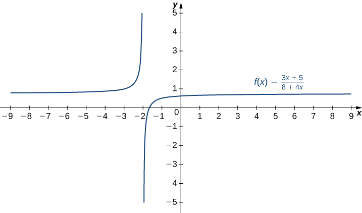
Sketch a graph of \(f(x)=\dfrac{3x+5}{8+4x}.\)

Hint

A line \(y=L\) is a horizontal asymptote of \(f\) if the limit as \(x→∞\) or the limit as \(x→−∞\) of \(f(x)\) is \(L\). A line \(x=a\) is a vertical asymptote if at least one of the one-sided limits of \(f\) as \(x→a\) is \(∞\) or \(−∞.\)

Answer

Example \(\PageIndex{3}\): Sketching a Rational Function with an Oblique Asymptote

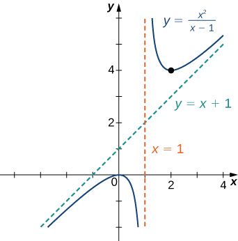
Sketch the graph of \(f(x)=\dfrac{x^2}{x−1}\)

Solution

Step 1: The domain of \(f\) is the set of all real numbers \(x\) except \(x=1.\)

Step 2: Find the intercepts. We can see that when \(x=0, \,f(x)=0,\) so \((0,0)\) is the only intercept.

Step 3: Evaluate the limits at infinity. Since the degree of the numerator is one more than the degree of the denominator, \(f\) must have an oblique asymptote. To find the oblique asymptote, use long division of polynomials to write

\(f(x)=\dfrac{x^2}{x−1}=x+1+\dfrac{1}{x−1}\).

Since \(\dfrac{1}{x−1}→0\) as \(x→±∞, f(x)\) approaches the line \(y=x+1\) as \(x→±∞\). The line \(y=x+1\) is an oblique asymptote for \(f\).

Step 4: To check for vertical asymptotes, look at where the denominator is zero. Here the denominator is zero at \(x=1.\) Looking at both one-sided limits as \(x→1,\) we find

\(\displaystyle \lim_{x→1^+}\frac{x^2}{x−1}=∞\) and \(\displaystyle \lim_{x→1^−}\frac{x^2}{x−1}=−∞.\)

Therefore, \(x=1\) is a vertical asymptote, and we have determined the behavior of \(f\) as \(x\) approaches \(1\) from the right and the left.

Step 5: Calculate the first derivative:

\(f′(x)=\dfrac{(x−1)(2x)−x^2(1)}{(x−1)^2}=\dfrac{x^2−2x}{(x−1)^2}.\)

We have \(f′(x)=0\) when \(x^2−2x=x(x−2)=0\). Therefore, \(x=0\) and \(x=2\) are critical points. Since \(f\) is undefined at \(x=1\), we need to divide the interval \((−∞,∞)\) into the smaller intervals \((−∞,0), (0,1), (1,2),\) and \((2,∞)\), and choose a test point from each interval to evaluate the sign of \(f′(x)\) in each of these smaller intervals. For example, let \(x=−1, x=\frac{1}{2}, x=\frac{3}{2}\), and \(x=3\) be the test points as shown in the following table.

Interval	Test Point	Sign of \(f'(x)=\dfrac{x^2−2x}{(x−1)^2}\)	Conclusion
\((−∞,0)\)	\(x=−1\)	(−)(−)/+=+	\(f\) is increasing.
\((0,1)\)	\(x=1/2\)	(+)(−)/+=−	\(f\) is decreasing.
\((1,2)\)	\(x=3/2\)	(+)(−)/+=−	\(f\) is decreasing.
\((2,∞)\)	\(x=3\)	(+)(+)/+=+	\(f\) is increasing.

From this table, we see that \(f\) has a local maximum at \(x=0\) and a local minimum at \(x=2\). The value of \(f\) at the local maximum is \(f(0)=0\) and the value of \(f\) at the local minimum is \(f(2)=4\). Therefore, \((0,0)\) and \((2,4)\) are important points on the graph.

Step 6. Calculate the second derivative:

\[\begin{align*} f''(x) &= \frac{(x−1)^2(2x−2)−2(x−1)(x^2−2x)}{(x−1)^4}\\[4pt]
&=\frac{2(x−1)[(x−1)^2−(x^2−2x)]}{(x−1)^4}\\[4pt]
&=\frac{2[x^2-2x+1−x^2+2x]}{(x−1)^3}\\[4pt]
&=\frac{2}{(x−1)^3}. \end{align*}\]

We see that \(f''(x)\) is never zero or undefined for \(x\) in the domain of \(f\). Since \(f\) is undefined at \(x=1\), to check concavity we just divide the interval \((−∞,∞)\) into the two smaller intervals \((−∞,1)\) and \((1,∞)\), and choose a test point from each interval to evaluate the sign of \(f''(x)\) in each of these intervals. The values \(x=0\) and \(x=2\) are possible test points as shown in the following table.

Interval	Test Point	Sign of \(f''(x)=\dfrac{2}{(x−1)^3}\)	Conclusion
\((−∞,1)\)	\(x=0\)	\(+/−=−\)	\(f\) is concave down.
\((1,∞)\)	\(x=2\)	\(+/+=+\)	\(f\) is concave up

From the information gathered, we arrive at the following graph for \(f.\)

Exercise \(\PageIndex{3}\)

Find the oblique asymptote for \(f(x)=\dfrac{3x^3−2x+1}{2x^2−4}\).

Hint

Use long division of polynomials.

Answer

\(y=\frac{3}{2}x\)

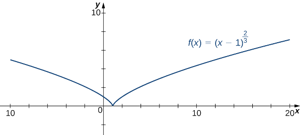
Example \(\PageIndex{4}\): Sketching the Graph of a Function with a Cusp

Sketch a graph of \(f(x)=(x−1)^{2/3}\)

Solution

Step 1: Since the cube-root function is defined for all real numbers \(x\) and \((x−1)^{2/3}=(\sqrt[3]{x−1})^2\), the domain of \(f\) is all real numbers.

Step 2: To find the \(y\)-intercept, evaluate \(f(0)\). Since \(f(0)=1,\) the \(y\)-intercept is \((0,1)\). To find the \(x\)-intercept, solve \((x−1)^{2/3}=0\). The solution of this equation is \(x=1\), so the \(x\)-intercept is \((1,0).\)

Step 3: Since \(\displaystyle \lim_{x→±∞}(x−1)^{2/3}=∞,\) the function continues to grow without bound as \(x→∞\) and \(x→−∞.\)

Step 4: The function has no vertical asymptotes.

Step 5: To determine where \(f\) is increasing or decreasing, calculate \(f′.\) We find

\[f′(x)=\frac{2}{3}(x−1)^{−1/3}=\frac{2}{3(x−1)^{1/3}}\]

This function is not zero anywhere, but it is undefined when \(x=1.\) Therefore, the only critical point is \(x=1.\) Divide the interval \((−∞,∞)\) into the smaller intervals \((−∞,1)\) and \((1,∞)\), and choose test points in each of these intervals to determine the sign of \(f′(x)\) in each of these smaller intervals. Let \(x=0\) and \(x=2\) be the test points as shown in the following table.

Interval	Test Point	Sign of \(f′(x)=\frac{2}{3(x−1)^{1/3}}\)	Conclusion
\((−∞,1)\)	\(x=0\)	\(+/−=−\)	\(f\) is decreasing
\((1,∞)\)	\(x=2\)	\(+/+=+\)	\(f\) is increasing

We conclude that \(f\) has a local minimum at \(x=1\). Evaluating \(f\) at \(x=1\), we find that the value of \(f\) at the local minimum is zero. Note that \(f′(1)\) is undefined, so to determine the behavior of the function at this critical point, we need to examine \(\displaystyle \lim_{x→1}f′(x).\) Looking at the one-sided limits, we have

\[\lim_{x→1^+}\frac{2}{3(x−1)^{1/3}}=∞\text{ and } \lim_{x→1^−}\frac{2}{3(x−1)^{1/3}}=−∞.\nonumber\]

Therefore, \(f\) has a cusp at \(x=1.\)

Step 6: To determine concavity, we calculate the second derivative of \(f:\)

\[f''(x)=−\dfrac{2}{9}(x−1)^{−4/3}=\dfrac{−2}{9(x−1)^{4/3}}.\]

We find that \(f''(x)\) is defined for all \(x\), but is undefined when \(x=1\). Therefore, divide the interval \((−∞,∞)\) into the smaller intervals \((−∞,1)\) and \((1,∞)\), and choose test points to evaluate the sign of \(f''(x)\) in each of these intervals. As we did earlier, let \(x=0\) and \(x=2\) be test points as shown in the following table.

Interval	Test Point	Sign of \(f''(x)=\dfrac{−2}{9(x−1)^{4/3}}\)	Conclusion
\((−∞,1)\)	\(x=0\)	\(−/+=−\)	\(f\) is concave down
\((1,∞)\)	\(x=2\)	\(−/+=−\)	\(f\) is concave down

From this table, we conclude that \(f\) is concave down everywhere. Combining all of this information, we arrive at the following graph for \(f\).

Exercise \(\PageIndex{4}\)

Consider the function \(f(x)=5−x^{2/3}\). Determine the point on the graph where a cusp is located. Determine the end behavior of \(f\).

Hint

A function \(f\) has a cusp at a point a if \(f(a)\) exists, \(f'(a)\) is undefined, one of the one-sided limits as \(x→a\) of \(f'(x)\) is \(+∞\), and the other one-sided limit is \(−∞.\)

Answer

The function \(f\) has a cusp at \((0,5)\), since \(\displaystyle \lim_{x→0^−}f′(x)=∞\) and \(\displaystyle \lim_{x→0^+}f′(x)=−∞\). For end behavior, \(\displaystyle \lim_{x→±∞}f(x)=−∞.\)

Key Concepts

• If \(c\) is a critical point of \(f\) and \(f'(x)>0\) for \(x<c\) and \(f'(x)<0\) for \(x>c\), then \(f\) has a local maximum at \(c\).
• If \(c\) is a critical point of \(f\) and \(f'(x)<0\) for \(x<c\) and \(f'(x)>0\) for \(x>c,\) then \(f\) has a local minimum at \(c\).
• If \(f''(x)>0\) over an interval \(I\), then \(f\) is concave up over \(I\).
• If \(f''(x)<0\) over an interval \(I\), then \(f\) is concave down over \(I\).
• If \(f'(c)=0\) and \(f''(c)>0\), then \(f\) has a local minimum at \(c\).
• If \(f'(c)=0\) and \(f''(c)<0\), then \(f\) has a local maximum at \(c\).
• If \(f'(c)=0\) and \(f''(c)=0\), then evaluate \(f'(x)\) at a test point \(x\) to the left of \(c\) and a test point \(x\) to the right of \(c\), to determine whether \(f\) has a local extremum at \(c\).

Glossary

concave down

if \(f\) is differentiable over an interval \(I\) and \(f'\) is decreasing over \(I\), then \(f\) is concave down over \(I\)

concave up

if \(f\) is differentiable over an interval \(I\) and \(f'\) is increasing over \(I\), then \(f\) is concave up over \(I\)

concavity

the upward or downward curve of the graph of a function

concavity test

suppose \(f\) is twice differentiable over an interval \(I\); if \(f''>0\) over \(I\), then \(f\) is concave up over \(I\); if \(f''<\) over \(I\), then \(f\) is concave down over \(I\)

first derivative test

let \(f\) be a continuous function over an interval \(I\) containing a critical point \(c\) such that \(f\) is differentiable over \(I\) except possibly at \(c\); if \(f'\) changes sign from positive to negative as \(x\) increases through \(c\), then \(f\) has a local maximum at \(c\); if \(f'\) changes sign from negative to positive as \(x\) increases through \(c\), then \(f\) has a local minimum at \(c\); if \(f'\) does not change sign as \(x\) increases through \(c\), then \(f\) does not have a local extremum at \(c\)

inflection point

if \(f\) is continuous at \(c\) and \(f\) changes concavity at \(c\), the point \((c,f(c))\) is an inflection point of \(f\)

second derivative test

suppose \(f'(c)=0\) and \(f'\)' is continuous over an interval containing \(c\); if \(f''(c)>0\), then \(f\) has a local minimum at \(c\); if \(f''(c)<0\), then \(f\) has a local maximum at \(c\); if \(f''(c)=0\), then the test is inconclusive

Contributors and Attributions

• Gilbert Strang (MIT) and Edwin “Jed” Herman (Harvey Mudd) with many contributing authors. This content by OpenStax is licensed with a CC-BY-SA-NC 4.0 license. Download for free at http://cnx.org.