2.1: Linear First Order Equations (Option 1- Variation of Parameters)

A first order differential equation is said to be linear if it can be written as

A first order differential equation that cannot be written like this is nonlinear. We say that Equation is homogeneous if ; otherwise it is nonhomogeneous. Since is obviously a solution of the homgeneous equation

we call it the trivial solution. Any other solution is nontrivial.

Example 2.1.1

The first order equations

are not in the form in Equation , but they are linear, since they can be rewritten as

Example 2.1.2

Here are some nonlinear first order equations:

General Solution of a Linear First Order Equation

To motivate a definition that we’ll need, consider the simple linear first order equation

From calculus we know that satisfies this equation if and only if

where is an arbitrary constant. We call a parameter and say that Equation defines a one–parameter family of functions. For each real number , the function defined by Equation is a solution of Equation on and ; moreover, every solution of Equation on either of these intervals is of the form Equation for some choice of . We say that Equation is the general solution of Equation .

We’ll see that a similar situation occurs in connection with any first order linear equation

that is, if and are continuous on some open interval then there’s a unique formula analogous to Equation that involves and a parameter and has the these properties:

• For each fixed value of , the resulting function of is a solution of Equation on .
• If is a solution of Equation on , then can be obtained from the formula by choosing appropriately.

We’ll call the general solution of Equation .

When this has been established, it will follow that an equation of the form

has a general solution on any open interval on which , , and are all continuous and has no zeros, since in this case we can rewrite Equation in the form Equation with and , which are both continuous on .

To avoid awkward wording in examples and exercises, we will not specify the interval when we ask for the general solution of a specific linear first order equation. Let’s agree that this always means that we want the general solution on every open interval on which and are continuous if the equation is of the form Equation , or on which , , and are continuous and has no zeros, if the equation is of the form Equation . We leave it to you to identify these intervals in specific examples and exercises.

For completeness, we point out that if , , and are all continuous on an open interval , but does have a zero in , then Equation may fail to have a general solution on in the sense just defined. Since this isn’t a major point that needs to be developed in depth, we will not discuss it further; however, see Exercise 2.1.44 for an example.

Homogeneous Linear First Order Equations

We begin with the problem of finding the general solution of a homogeneous linear first order equation. The next example recalls a familiar result from calculus.

Example 2.1.3

Let be a constant.

1. Find the general solution of
2. Solve the initial value problem

Solution a

(a) You already know from calculus that if is any constant, then satisfies Equation . However, let’s pretend you’ve forgotten this, and use this problem to illustrate a general method for solving a homogeneous linear first order equation.

We know that Equation has the trivial solution . Now suppose is a nontrivial solution of Equation . Then, since a differentiable function must be continuous, there must be some open interval on which has no zeros. We rewrite Equation as

Figure 2.1.1 : Solutions of ,

for in . Integrating this shows that

where is an arbitrary constant. Therefore we can rewrite as

 

This shows that every nontrivial solution of Equation is of the form for some nonzero constant . Since setting yields the trivial solution, all solutions of Equation are of the form Equation . Conversely, Equation is a solution of Equation for every choice of , since differentiating Equation yields .

Solution b

Imposing the initial condition yields , so and

Figure 2.1.1 show the graphs of this function with , , and various values of .

Example 2.1.4

a. Find the general solution of

b. Solve the initial value problem

Solution a

We rewrite Equation as

where is restricted to either or . If is a nontrivial solution of Equation , there must be some open interval I on which has no zeros. We can rewrite Equation as

for in . Integrating shows that

We can rewrite this result more simply as

 

We have now shown that every solution of Equation is given by Equation for some choice of . (Even though we assumed that was nontrivial to derive Equation , we can get the trivial solution by setting in Equation .) Conversely, any function of the form Equation is a solution of Equation , since differentiating Equation yields

and substituting this and Equation into Equation yields

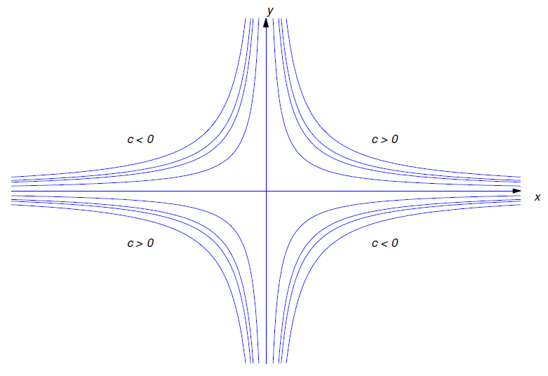
Figure 2.1.2 shows the graphs of some solutions corresponding to various values of

Solution b

Imposing the initial condition in Equation yields . Therefore the solution of Equation is

The interval of validity of this solution is .

The results in Examples and are special cases of the next theorem.

Theorem 2.1.1

If is continuous on then the general solution of the homogeneous equation

on is

where

is any antiderivative of on that is

Figure 2.1.2 : Solutions of on and

Proof

If , differentiating and using Equation shows that

so ; that is, is a solution of Equation , for any choice of .

Now we’ll show that any solution of Equation can be written as for some constant . The trivial solution can be written this way, with . Now suppose is a nontrivial solution. Then there’s an open subinterval of on which has no zeros. We can rewrite Equation as

for in . Integrating Equation and recalling Equation yields

where is a constant. This implies that

Since is defined for all in and an exponential can never equal zero, we can take , so has zeros on , so we can rewrite the last equation as , where

REMARK: Rewriting a first order differential equation so that one side depends only on and and the other depends only on is called separation of variables. We did this in Examples 2.1.3 and 2.1.4 , and in rewriting Equation and Equation ​. We will apply this method to nonlinear equations in Section 2.2.

Linear Nonhomogeneous First Order Equations

We’ll now solve the nonhomogeneous equation

When considering this equation we call

the complementary equation.

We’ll find solutions of Equation in the form , where is a nontrivial solution of the complementary equation and is to be determined. This method of using a solution of the complementary equation to obtain solutions of a nonhomogeneous equation is a special case of a method called variation of parameters, which you’ll encounter several times in this book. (Obviously, can’t be constant, since if it were, the left side of Equation would be zero. Recognizing this, the early users of this method viewed as a “parameter” that varies; hence, the name “variation of parameters.”)

If

Substituting these expressions for and into Equation yields

which reduces to

since is a solution of the complementary equation; that is,

In the proof of Theorem 2.2.1 we saw that has no zeros on an interval where is continuous. Therefore we can divide Equation through by to obtain

We can integrate this (introducing a constant of integration), and multiply the result by to get the general solution of Equation . Before turning to the formal proof of this claim, let’s consider some examples.

Example 2.1.5

Find the general solution of

By applying a of Example 2.1.3 with , we see that is a solution of the complementary equation . Therefore we seek solutions of Equation in the form , so that

Therefore is a solution of Equation if and only if

Therefore

Figure 2.1.3 : A direction field and integral curves for

and

is the general solution of Equation .

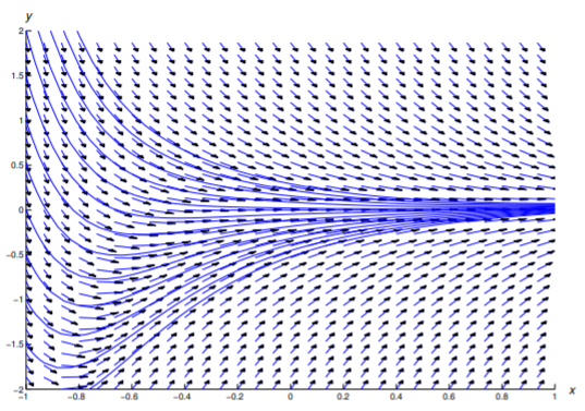
Figure 2.1.3 shows a direction field and some integral curves for Equation .

Example 2.1.6

Find the general solution

Solve the initial value problem

Here and are both continuous except at the points , where is an integer. Therefore we seek solutions of Equation on the intervals . We need a nontrival solution of the complementary equation; thus, must satisfy , which we rewrite as

Integrating this yields

where we take the constant of integration to be zero since we need only one function that satisfies Equation . Clearly is a suitable choice. Therefore we seek solutions of Equation in the form

so that

and

Therefore is a solution of Equation if and only if

Integrating this yields

is the general solution of Equation on every interval ( integer).

b. Imposing the initial condition in Equation yields

Thus,

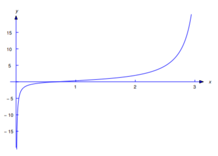
is a solution of Equation . The interval of validity of this solution is ; Figure 2.1.4 shows its graph.

Figure 2.1.4 : Solution of

REMARK: It wasn’t necessary to do the computations and in Example 2.1.6 , since we showed in the discussion preceding Example 2.1.5 that if where , then . We did these computations so you would see this happen in this specific example. We recommend that you include these “unnecesary” computations in doing exercises, until you’re confident that you really understand the method. After that, omit them.

We summarize the method of variation of parameters for solving

as follows:

a. Find a function such that

For convenience, take the constant of integration to be zero.

b. Write

to remind yourself of what you’re doing.

c. Write and solve for ; thus, .

d. Integrate to obtain , with an arbitrary constant of integration.

e. Substitute into Equation to obtain .

To solve an equation written as

we recommend that you divide through by to obtain an equation of the form Equation and then follow this procedure.

Solutions in Integral Form

Sometimes the integrals that arise in solving a linear first order equation can’t be evaluated in terms of elementary functions. In this case the solution must be left in terms of an integral.

Example 2.1.7

Find the general solution of

Solve the initial value problem

a. To apply variation of parameters, we need a nontrivial solution of the complementary equation; thus, , which we rewrite as

Integrating this and taking the constant of integration to be zero yields

We choose and seek solutions of Equation in the form , where

Therefore

but we can’t simplify the integral on the right because there’s no elementary function with derivative equal to . Therefore the best available form for the general solution of Equation is

b. Since the initial condition in Equation is imposed at , it is convenient to rewrite Equation as

Setting and here shows that . Therefore the solution of the initial value problem is

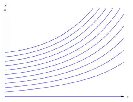
For a given value of and each fixed , the integral on the right can be evaluated by numerical methods. An alternate procedure is to apply the numerical integration procedures discussed in Chapter 3 directly to the initial value problem Equation . Figure 2.1.5 shows graphs of of Equation for several values of .

Figure 2.1.5 : Solution of

An Existence and Uniqueness Theorem

The method of variation of parameters leads to this theorem.

Theorem 2.1.2 Existence and Uniqueness Theorem

Suppose and are continuous on an open interval and let be any nontrivial solution of the complementary equation

on . Then:

1. The general solution of the nonhomogeneous equation on is
2. If is an arbitrary point in and is an arbitrary real number then the initial value problem has the unique solution on

Proof

(a) To show that Equation is the general solution of Equation on , we must prove that:

1. If is any constant, the function in Equation is a solution of Equation on .
2. If is a solution of Equation on then is of the form Equation for some constant .

To prove (i), we first observe that any function of the form Equation is defined on , since and are continuous on . Differentiating Equation yields

Since , this and Equation imply that

which implies that is a solution of Equation .

To prove (ii), suppose is a solution of Equation on . From the proof of Theorem 2.1.1, we know that has no zeros on , so the function is defined on . Moreover, since

Integrating yields

which implies Equation , since .

(b) We’ve proved (a), where in Equation is an arbitrary antiderivative of . Now it is convenient to choose the antiderivative that equals zero when , and write the general solution of Equation as

Since

we see that if and only if .