14.4: Constant coefficient second order linear ODEs

Solving Constant Coefficient Equations

Suppose we have the problem

$$y'' - 6y' + 8y = 0, y(0) = -2, y'(0) = 6 \nonumber$$

This is a second order linear homogeneous equation with constant coefficients. Constant coefficients means that the functions in front of $y''$, $y'$, and $y$ are constants and do not depend on $x$.

To guess a solution, think of a function that you know stays essentially the same when we differentiate it, so that we can take the function and its derivatives, add some multiples of these together, and end up with zero.

Let us try$^{1}$ a solution of the form $y = e^{rx}$. Then $y' = re^{rx}$ and $y'' = r^2e^{rx}$. Plug in to get

$$\begin{align}\begin{aligned} y''-6y'+8y & = 0 , \\ \underbrace{r^2 e^{rx}}_{y''} -6 \underbrace{r e^{rx}}_{y'}+8 \underbrace{e^{rx}}_{y} & = 0 , \\ r^2 -6 r +8 & = 0 \qquad \text{(divide through by } e^{rx} \text{)},\\ (r-2)(r-4) & = 0 .\end{aligned}\end{align} \nonumber$$

Hence, if $r = 2$ or $r = 4$, then $e^{rx}$ is a solution. So let $y_1 = e^{2x}$ and $y_2 = e^{4x}$.

Exercise $\PageIndex{1}$

Check that $y_1$ and $y_2$ are solutions.

Solution

The functions $e^{2x}$ and $e^{4x}$ are linearly independent. If they were not linearly independent we could write $e^{4x} = Ce^{2x}$ for some constant $C$, implying that $e^{2x} = C$for all $x$, which is clearly not possible. Hence, we can write the general solution as

$$y = C_1e^{2x} + C_2e^{4x} \nonumber$$

We need to solve for $C_1$ and $C_2$. To apply the initial conditions we first find $y' = 2C_1e^{2x} + 4C_2e^{4x}$. We plug in $x = 0$ and solve.

$$\begin{align}\begin{aligned} -2 &= y(0) = C_1 + C_2 \\ 6 &= y'(0) = 2C_1 + 4C_2 \end{aligned}\end{align} \nonumber$$

Either apply some matrix algebra, or just solve these by high school math. For example, divide the second equation by 2 to obtain $3 = C_1 + 2C_2$, and subtract the two equations to get $5 = C_2$. Then $C_1 = -7$ as $-2 = C_1 + 5$. Hence, the solution we are looking for is

$$y = -7e^{2x} + 5e^{4x} \nonumber$$

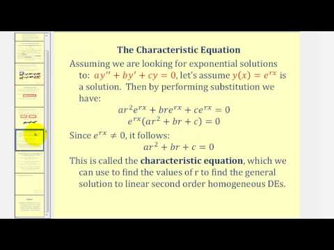
Let us generalize this example into a method. Suppose that we have an equation

$$\label{eq:6}ay'' +by' +cy = 0,$$

where $a, b, c$ are constants. Try the solution $y = e^{rx}$ to obtain

$$ar^2 e^{rx} + bre^{rx} + ce^{rx} = 0 \nonumber$$

Divide by $e^{rx}$ to obtain the so-called characteristic equation of the ODE:

$$ar^2 + br + c = 0 \nonumber$$

Solve for the $r$ by using the quadratic formula.

$$r_1, r_2 = \dfrac {-b \pm \sqrt {b^2 - 4ac}}{2a} \nonumber$$

Therefore, we have $e^{r_1x}$ and $e^{r_2x}$ as solutions. There is still a difficulty if $r_1 = r_2$, but it is not hard to overcome.

Theorem $\PageIndex{1}$

Suppose that $r_1$ and $r_2$ are the roots of the characteristic equation.

If $r_1$ and $r_2$ are distinct and real (when $b^2 - 4ac > 0$ ), then $\eqref{eq:6}$ has the general solution

$$y = C_1e^{r_1x} + C_2e^{r_2x} \nonumber$$

If $r_1 = r_2$ (happens when $b^2 - 4ac = 0$ ), then $\eqref{eq:6}$ has the general solution

$$y = (C_1 + C_2x)e^{r_1x} \nonumber$$

For another example of the first case, take the equation $y'' - k^2y = 0$. Here the characteristic equation is $r^2 - k^2 = 0$ or $(r - k)(r + k) = 0$. Consequently, $e^{-kx}$ and $e^{kx}$ are the two linearly independent solutions.

Below is a video on the characteristic equation of a differential equation.

Example $\PageIndex{1}$

Solve

$$y''-k^{2}y=0. \nonumber$$

Solution

The characteristic equation is $r^{2}-k^{2}=0$ or $(r-k)(r+k)=0$. Consequently, $e^{-kx}$ and $e^{kx}$ are the two linearly independent solutions, and the general solution is $$y=C_{1}e^{kx}+C_{2}e_{-kx}. \nonumber$$

Since $\cosh s=\frac{e^{s}+e^{-s}}{2}$ and $\sinh s=\frac{e^{s}-e^{-s}}{2}$, we can also write the general solution as $$y=D_{1}\cosh (kx)+D_{2}\sinh (kx). \nonumber$$

Below is a video on finding the finding the general solution to a differential equation.

Example $\PageIndex{2}$:

Find the general solution of $$y'' - 8y' + 16y = 0 \nonumber$$

Solution

The characteristic equation is $r^2 - 8r + 16 = {( r - 4)}^2 = 0$. The equation has a double root $r_1 = r_2 = 4$. The general solution is, therefore,

$$y = (C_1 + C_2x)e^{4x} = C_1e^{4x} + C_2xe^{4x} \nonumber$$

Below is a video on finding the general solution to a differential equation involving two real irrational roots.

Exercise $\PageIndex{2}$: Linear Independence

Check that $e^{4x}$ and $xe^{4x}$ are linearly independent.

Answer

That $e^{4x}$ solves the equation is clear. If $xe^{4x}$ solves the equation, then we know we are done. Let us compute $y' = e^{4x} + 4xe^{4x}$ and $y'' = 8e^{4x} + 16xe^{4x}$. Plug in

$$y'' - 8y' + 16y = 8e^{4x} + 16xe^{4x} - 8(e^{4x} + 4xe^{4x} ) + 16xe^{4x} = 0 \nonumber$$

We should note that in practice, doubled root rarely happens. If coefficients are picked truly randomly we are very unlikely to get a doubled root.

Below is a video on finding the the general solution to a differential equation.

Let us give a short proof for why the solution $xe^{rx}$ works when the root is doubled. This case is really a limiting case of when the two roots are distinct and very close. Note that $\frac {e^r2^x - e^x1^x}{r_2 - r_1}$ is a solution when the roots are distinct. When we take the limit as $r_1$ goes to $r_2$, we are really taking the derivative of $e^{rx}$ using $r$ as the variable. Therefore, the limit is $xe^{rx}$, and hence this is a solution in the doubled root case.

Below is a video on finding the solution to a differential equation involving repeated roots.

Complex numbers and Euler’s formula

It may happen that a polynomial has some complex roots. For example, the equation $r^2 + 1 = 0$ has no real roots, but it does have two complex roots. Here we review some properties of complex numbers.

Complex numbers may seem a strange concept, especially because of the terminology. There is nothing imaginary or really complicated about complex numbers. A complex number is simply a pair of real numbers, $(a, b)$. We can think of a complex number as a point in the plane. We add complex numbers in the straightforward way, $(a, b) + (c, d) = (a + c, b + d)$. We define multiplication by

$$(a,b) \times (c,d) \overset{\text{def}}{=} (ac-bd,ad+bc) . \nonumber$$

It turns out that with this multiplication rule, all the standard properties of arithmetic hold. Further, and most importantly $( 0, 1) \times (0,1) = (-1, 0 )$.

Generally we just write $(a, b)$ as $(a + ib)$, and we treat $i$ as if it were an unknown. We do arithmetic with complex numbers just as we would with polynomials. The property we just mentioned becomes $i^2 = -1$. So whenever we see $i^2$, we replace it by $-1$. The numbers $i$ and $-i$ are the two roots of $r^2 + 1 = 0$.

Note that engineers often use the letter $j$ instead of $i$ for the square root of $-1$. We will use the mathematicians’ convention and use $i$.

Exercise $\PageIndex{3}$

Make sure you understand (that you can justify) the following identities:

1. $i^2 = -1, i^3 = -1, i^4 = 1$,
2. $\frac {1}{i} = -i$,
3. $(3 -7i)(-2 -9i) = \dots = -69 - 13i$,
4. $(3 - 2i)(3 + 2i) = 3^2 - {(2i)}^2 = 3^2 + 2^2 = 13$,
5. $\frac {1}{3-2i} = \frac {1}{3-2i} \frac {3+2i}{3+2i} = \frac{3+2i}{13} = \frac {3}{13} + \frac{2}{13} i$.

We can also define the exponential $e^{a+ib}$ of a complex number. We do this by writing down the Taylor series and plugging in the complex number. Because most properties of the exponential can be proved by looking at the Taylor series, these properties still hold for the complex exponential. For example the very important property: $e^{x+y} = e^xe^y$. This means that $e^{a+ib} = e^ae^{ib}$. Hence if we can compute $e^{ib}$, we can compute $e^{a+ib}$. For $e^{ib}$ we use the so-called Euler’s formula.

Theorem $\PageIndex{2}$

Euler's Formula

$$e^{i\theta} = \cos \theta + i \sin \theta \quad { \it{~and~ } }\quad e^{-i\theta} = \cos \theta - i\sin \theta \nonumber$$

In other words, $e^{a+ib}=e^{a}(\cos (b)+i\sin (b))=e^{a}\cos (b)+ie^{a}\sin (b)$.

Exercise $\PageIndex{4}$:

Using Euler’s formula, check the identities:

$$\cos \theta = \frac { e^{i \theta} + e^{-i \theta}}{2} \quad\text{and}\quad \sin \theta = \frac { e^{i \theta} - e^{-i \theta}}{2i} \nonumber$$

Exercise $\PageIndex{5}$

Double angle identities: Start with $e^{i (2 \theta)} = {(e^{i \theta})}^2$. Use Euler on each side and deduce:

Answer

$$\cos (2 \theta) = {\cos}^2 \theta - {\sin}^2 \theta \quad\text{and}\quad \sin (2 \theta) = 2 \sin \theta \cos \theta \nonumber$$

For a complex number $a + ib$ we call $a$ the real part and $b$ the imaginary part of the number. Often the following notation is used,

$$\text{Re}(a + ib) =a \quad\text{and}\quad \text{Im} (a + ib) = b \nonumber$$

Complex roots

Suppose that the equation $ay'' + by' + cy = 0$ has the characteristic equation $ar^2 + br + c = 0$ that has complex roots. By the quadratic formula, the roots are $\dfrac{-b \pm \sqrt {b^2 - 4ac}}{2a}$. These roots are complex if $b^2 - 4ac < 0$. In this case the roots are

$$r_1, r_2 = \frac {-b}{2a} \pm i \dfrac { \sqrt {4ac - b^2}}{2a} \nonumber$$

As you can see, we always get a pair of roots of the form $\alpha \pm i \beta$. In this case we can still write the solution as

$$y = C_1e^{(\alpha + i \beta )x} + C_2e^{(\alpha - i\beta)x} \nonumber$$

However, the exponential is now complex valued. We would need to allow $C_1$ and $C_2$ to be complex numbers to obtain a real-valued solution (which is what we are after). While there is nothing particularly wrong with this approach, it can make calculations harder and it is generally preferred to find two real-valued solutions.

Here we can use Euler’s formula. Let

$$y_1 = e^{(\alpha + i\beta)x} \quad\text{and}\quad y_2 = e^{( \alpha - i \beta ) x} \nonumber$$

Then note that

$$\begin{align}\begin{aligned} y_1 &= e^{ax} \cos (\beta x) + ie^{ax} \sin ( \beta x) \\ y_2 &= e^{ax} \cos (\beta x) - ie^{ax} \sin (\beta x) \end{aligned}\end{align} \nonumber$$

Linear combinations of solutions are also solutions. Hence,

$$\begin{align}\begin{aligned} y_3 &= \frac {y_1 + y_2}{2} = e^{ax} \cos (\beta x) \\ y_4 &= \frac {y_1 - y_2}{2i} = e^{ax} \sin (\beta x) \end{aligned}\end{align} \nonumber$$

are also solutions. Furthermore, they are real-valued. It is not hard to see that they are linearly independent (not multiples of each other). Therefore, we have the following theorem.

Theorem $\PageIndex{3}$

For the homegneous second order ODE

$$ay'' + by' + cy = 0 \nonumber$$

If the characteristic equation has the roots $\alpha \pm i \beta$ (when $b^2 - 4ac < 0$), then the general solution is

$$y = C_1e^{ax} \cos (\beta x) + C_2e^{ax} \sin (\beta x) \nonumber$$

Below is a video on finding the solution to a differential equation using the principal of superposition.

Example $\PageIndex{3}$

Find the general solution of $y'' + k^2 y = 0$, for a constant $k > 0$.

Solution

The characteristic equation is $r^2 + k^2 = 0$. Therefore, the roots are $r = \pm ik$ and by the theorem we have the general solution

$$y = C_1 \cos (kx) + C_2 \sin (kx) \nonumber$$

Below is a video on finding the solution to a differential equation involving complex roots.

Example $\PageIndex{4}$

Find the solution of $y'' - 6y' + 13y = 0, y(0) = 0, y'(0) = 10.$

Solution

The characteristic equation is $r^2 - 6r + 13 = 0$. By completing the square we get ${(r -3)}^2 + 2^2 = 0$ and hence the roots are $r = 3 \pm 2i$. By the theorem we have the general solution

$$y = C_1e^{3x} \cos (2x) + C_2 e^{3x} \sin (2x) \nonumber$$

To find the solution satisfying the initial conditions, we first plug in zero to get

$$0 = y(0) = C_1e^0 \cos 0 + C_2e^0 \sin 0 = C_1 \nonumber$$

Hence $C_1 = 0$ and $y = C_2e^{3x} \sin (2x)$. We differentiate

$$y' = 3C_2 e^{3x} \sin (2x) + 2C_2e^{3x} \cos (2x) \nonumber$$

We again plug in the initial condition and obtain $10 = y'(0) = 2C_2$, or $C_2 = 5$. Hence the solution we are seeking is

$$y = 5e^{3x} \sin (2x) \nonumber$$

Below is a video on finding the solution to an initial value problem.

Below is a video on finding the solution to a differential equation given initial values.

Below is another video on finding the solution to a differential equation given initial values.

 

Footnotes

[1] Making an educated guess with some parameters to solve for is such a central technique in differential equations, that people sometimes use a fancy name for such a guess: ansatz, German for “initial placement of a tool at a work piece.” Yes, the Germans have a word for that.