4.3: The First Derivative Test

Learning Objectives

• Explain how the sign of the first derivative affects the shape of a function’s graph.
• State the first derivative test for critical points.
• Find local extrema using the First Derivative Test.

Earlier in this chapter we stated that if a function \(f\) has a local extremum at a point \(c\), then \(c\) must be a critical point of \(f\). However, a function is not guaranteed to have a local extremum at a critical point. For example, \(f(x)=x^3\) has a critical point at \(x=0\) since \(f'(x)=3x^2\) is zero at \(x=0\), but \(f\) does not have a local extremum at \(x=0\). Using the results from the previous section, we are now able to determine whether a critical point of a function actually corresponds to a local extreme value. In this section, we also see how the second derivative provides information about the shape of a graph by describing whether the graph of a function curves upward or curves downward.

The First Derivative Test

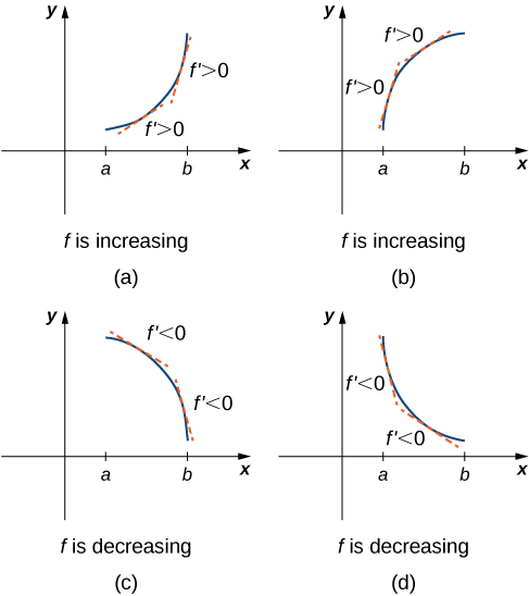
Corollary \(3\) of the Mean Value Theorem showed that if the derivative of a function is positive over an interval \(I\) then the function is increasing over \(I\). On the other hand, if the derivative of the function is negative over an interval \(I\), then the function is decreasing over \(I\) as shown in the following figure.

Figure \(\PageIndex{1}\): Both functions are increasing over the interval \((a,b)\). At each point \(x\), the derivative \(f'(x)>0\). Both functions are decreasing over the interval \((a,b)\). At each point \(x\), the derivative \(f'(x)<0.\)

A continuous function \(f\) has a local maximum at point \(c\) if and only if \(f\) switches from increasing to decreasing at point \(c\). Similarly, \(f\) has a local minimum at \(c\) if and only if \(f\) switches from decreasing to increasing at \(c\). If \(f\) is a continuous function over an interval \(I\) containing \(c\) and differentiable over \(I\), except possibly at \(c\), the only way \(f\) can switch from increasing to decreasing (or vice versa) at point \(c\) is if \(f'\) changes sign as \(x\) increases through \(c\). If \(f\) is differentiable at \(c\), the only way that \(f'\) can change sign as \(x\) increases through \(c\) is if \(f'(c)=0\). Therefore, for a function \(f\) that is continuous over an interval \(I\) containing \(c\) and differentiable over \(I\), except possibly at \(c\), the only way \(f\) can switch from increasing to decreasing (or vice versa) is if \(f'(c)=0\) or \(f'(c)\) is undefined. Consequently, to locate local extrema for a function \(f\), we look for points \(c\) in the domain of \(f\) such that \(f'(c)=0\) or \(f'(c)\) is undefined. Recall that such points are called critical points of \(f\).

Note that \(f\) need not have a local extrema at a critical point. The critical points are candidates for local extrema only. In Figure \(\PageIndex{2}\), we show that if a continuous function \(f\) has a local extremum, it must occur at a critical point, but a function may not have a local extremum at a critical point. We show that if \(f\) has a local extremum at a critical point, then the sign of \(f'\) switches as \(x\) increases through that point.

Figure \(\PageIndex{2}\): The function \(f\) has four critical points: \(a,b,c\),and \(d\). The function \(f\) has local maxima at \(a\) and \(d\), and a local minimum at \(b\). The function \(f\) does not have a local extremum at \(c\). The sign of \(f'\) changes at all local extrema.

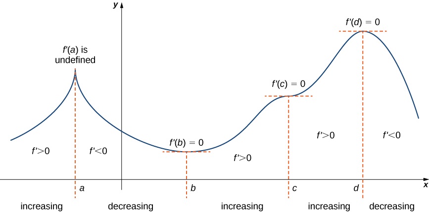
Using Figure \(\PageIndex{2}\), we summarize the main results regarding local extrema.

• If a continuous function \(f\) has a local extremum, it must occur at a critical point \(c\).
• The function has a local extremum at the critical point \(c\) if and only if the derivative \(f'\) switches sign as \(x\) increases through \(c\).
• Therefore, to test whether a function has a local extremum at a critical point \(c\), we must determine the sign of \(f'(x)\) to the left and right of \(c\).

This result is known as the first derivative test.

First Derivative Test

Suppose that \(f\) is a continuous function over an interval \(I\) containing a critical point \(c\). If \(f\) is differentiable over \(I\), except possibly at point \(c\), then \(f(c)\) satisfies one of the following descriptions:

1. If \(f'\) changes sign from positive when \(x<c\) to negative when \(x>c\), then \(f(c)\) is a local maximum of \(f\).
2. If \(f'\) changes sign from negative when \(x<c\) to positive when \(x>c\), then \(f(c)\) is a local minimum of \(f\).
3. If \(f'\) has the same sign for \(x<c\) and \(x>c\), then \(f(c)\) is neither a local maximum nor a local minimum of \(f\)

Now let’s look at how to use this strategy to locate all local extrema for particular functions.

Example \(\PageIndex{1}\): Using the First Derivative Test to Find Local Extrema

Use the first derivative test to find the location of all local extrema for \(f(x)=x^3−3x^2−9x−1.\) Use a graphing utility to confirm your results.

Solution

Step 1. The derivative is \(f'(x)=3x^2−6x−9.\) To find the critical points, we need to find where \(f'(x)=0.\) Factoring the polynomial, we conclude that the critical points must satisfy

\[3(x^2−2x−3)=3(x−3)(x+1)=0. \nonumber \]

Therefore, the critical points are \(x=3,−1.\) Now divide the interval \((−∞,∞)\) into the smaller intervals \((−∞,−1),(−1,3)\) and \((3,∞).\)

Step 2. Since \(f'\) is a continuous function, to determine the sign of \(f'(x)\) over each subinterval, it suffices to choose a point over each of the intervals \((−∞,−1),(−1,3)\) and \((3,∞)\) and determine the sign of \(f'\) at each of these points. For example, let’s choose \(x=−2\), \(x=0\), and \(x=4\) as test points.

Table: \(\PageIndex{1}\): First Derivative Test for \(f(x)=x^3−3x^2−9x−1.\)

Interval	Test Point	Sign of \(f'(x)=3(x−3)(x+1)\) at Test Point	Conclusion
\((−∞,−1)\)	\(x=−2\)	(+)(−)(−)=+	\(f\) is increasing.
\((−1,3)\)	\(x=0\)	(+)(−)(+)=-	\(f\) is decreasing.
\((3,∞)\)	\(x=4\)	(+)(+)(+)=+	\(f\) is increasing.

Step 3. Since \(f'\) switches sign from positive to negative as \(x\) increases through \(-1\), \(f\) has a local maximum at \(x=−1\). Since \(f'\) switches sign from negative to positive as \(x\) increases through \(3\), \(f\) has a local minimum at \(x=3\). These analytical results agree with the following graph.

Figure \(\PageIndex{3}\): The function \(f\) has a maximum at \(x=−1\) and a minimum at \(x=3\)

Exercise \(\PageIndex{1}\)

Use the first derivative test to locate all local extrema for \(f(x)=−x^3+\frac{3}{2}x^2+18x.\)

Hint

Find all critical points of \(f\) and determine the signs of \(f'(x)\) over particular intervals determined by the critical points.

Answer

\(f\) has a local minimum at \(−2\) and a local maximum at \(3\).

Example \(\PageIndex{2}\): Using the First Derivative Test

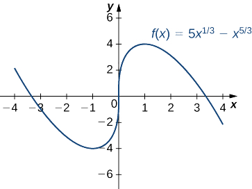
Use the first derivative test to find the location of all local extrema for \(f(x)=5x^{1/3}−x^{5/3}.\) Use a graphing utility to confirm your results.

Solution

Step 1. The derivative is

\[f'(x)=\frac{5}{3}x^{−2/3}−\frac{5}{3}x^{2/3}=\frac{5}{3x^{2/3}}−\frac{5x^{2/3}}{3}=\frac{5−5x^{4/3}}{3x^{2/3}}=\frac{5(1−x^{4/3})}{3x^{2/3}}.\nonumber \]

The derivative \(f'(x)=0\) when \(1−x^{4/3}=0.\) Therefore, \(f'(x)=0\) at \(x=±1\). The derivative \(f'(x)\) is undefined at \(x=0.\) Therefore, we have three critical points: \(x=0\), \(x=1\), and \(x=−1\). Consequently, divide the interval \((−∞,∞)\) into the smaller intervals \((−∞,−1),\,(−1,0),\,(0,1)\), and \((1,∞)\).

Step 2: Since \(f'\) is continuous over each subinterval, it suffices to choose a test point \(x\) in each of the intervals from step 1 and determine the sign of \(f'\) at each of these points. The points \(x=−2,\,x=−\frac{1}{2},\,x=\frac{1}{2}\), and \(x=2\) are test points for these intervals.

Table: \(\PageIndex{2}\): First Derivative Test for \(f(x)=5x^{1/3}−x^{5/3}.\)

Interval	Test Point	Sign of \(f'(x)=\frac{5(1−x^{4/3})}{3x^{2/3}}\) at Test Point	Conclusion
\((−∞,−1)\)	\(x=−2\)	\(\frac{(+)(−)}{+}=−\)	\(f\) is decreasing.
\((−1,0)\)	\(x=−\frac{1}{2}\)	\(\frac{(+)(+)}{+}=+\)	\(f\) is increasing.
\((0,1)\)	\(x=\frac{1}{2}\)	\(\frac{(+)(+)}{+}=+\)	\(f\) is increasing.
\((1,∞)\)	\(x=2\)	\(\frac{(+)(−)}{+}=−\)	\(f\) is decreasing.

Step 3: Since \(f\) is decreasing over the interval \((−∞,−1)\) and increasing over the interval \((−1,0)\), \(f\) has a local minimum at \(x=−1\). Since \(f\) is increasing over the interval \((−1,0)\) and the interval \((0,1)\), \(f\) does not have a local extremum at \(x=0\). Since \(f\) is increasing over the interval \((0,1)\) and decreasing over the interval \((1,∞)\), \(f\) has a local maximum at \(x=1\). The analytical results agree with the following graph.

Figure \(\PageIndex{4}\): The function \(f\) has a local minimum at \(x=−1\) and a local maximum at \(x=1\)

Exercise \(\PageIndex{2}\)

Use the first derivative test to find all local extrema for \(f(x)=\dfrac{3}{x−1}\).

Hint

The only critical point of \(f\) is \(x=1.\)

Answer

\(f\) has no local extrema because \(f'\) does not change sign at \(x=1\).