4.3: Linear Programming - Maximization Applications

Learning Objectives

In this section, you will learn to:

• Recognize the typical form of a linear programming problem.
• Formulate maximization linear programming problems.
• Graph feasible regions for maximization linear programming problems.
• Determine optimal solutions for maximization linear programming problems.

Prerequisite Skills

Before you get started, take this prerequisite quiz.

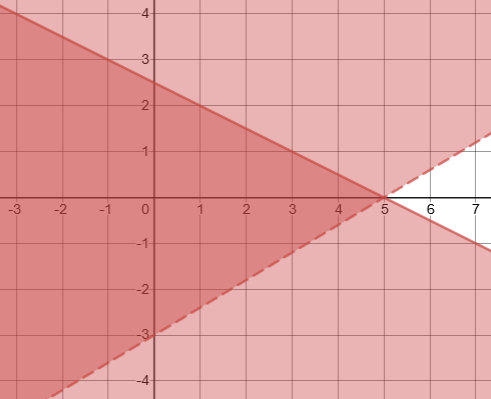
1. Graph this system of inequalities:

\(\left\{\begin{array} {l} 2x+4y\leq 10\\3x−5y<15\end{array}\right.\)

Click here to check your answer

If you missed this problem, review Section 4.2. (Note that this will open in a new window.)

 

2. Graph this system of inequalities:

\(\left\{\begin{array} {l} y\leq 2x+1\\y\leq-3x+6\\x\geq0\\y\geq0\end{array}\right.\)

Click here to check your answer

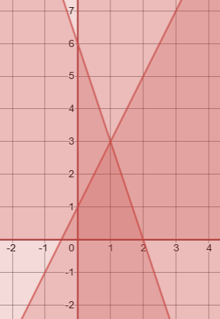
(The solution is in the center region.)

If you missed this problem, review Section 4.2. (Note that this will open in a new window.)

Application problems in business, economics, and social and life sciences often ask us to make decisions on the basis of certain conditions. The conditions or constraints often take the form of inequalities. In this section, we will begin to formulate, analyze, and solve such problems, at a simple level, to understand the many components of such a problem.

A typical linear programming problem consists of finding an extreme value of a linear function subject to certain constraints. We are either trying to maximize or minimize the value of this linear function, such as to maximize profit or revenue, or to minimize cost. That is why these linear programming problems are classified as maximization or minimization problems, or just optimization problems. The function we are trying to optimize is called an objective function, and the conditions that must be satisfied are called constraints.

When we graph all constraints, the area of the graph that satisfies all constraints is called the feasible region. The Fundamental Theorem of Linear Programming states that the maximum (or minimum) value of the objective function always takes place at the vertices of the feasible region.  We call these vertices critical points.  These are found using any methods from Chapter 3 as we are looking for the points where any two of the boundary lines intersect. 

A typical example is to maximize profit from producing several products, subject to limitations on materials or resources needed for producing these items; the problem requires us to determine the amount of each item produced. Another type of problem involves scheduling; we need to determine how much time to devote to each of several activities in order to maximize income from (or minimize cost of) these activities, subject to limitations on time and other resources available for each activity.

In this chapter, we will work with problems that involve only two variables, and therefore, can be solved by graphing. Here are the steps we'll follow:

The Maximization Linear Programming Problems

1. Define the unknowns.
2. Write the objective function that needs to be maximized.
3. Write the constraints.
   1. For the standard maximization linear programming problems, constraints are of the form: \(ax + by ≤ c\)
   2. Since the variables are non-negative, we include the constraints: \(x ≥ 0\); \(y ≥ 0\).
4. Graph the constraints.
5. Shade the feasible region.
6. Find the corner points.
7. Find the value of the objective function at each corner point to determine the corner point that gives the maximum value.

Example \(\PageIndex{1}\)

Niki holds two part-time jobs, Job I and Job II. She never wants to work more than a total of 12 hours a week. She has determined that for every hour she works at Job I, she needs 2 hours of preparation time, and for every hour she works at Job II, she needs one hour of preparation time, and she cannot spend more than 16 hours for preparation.

If Niki makes $40 an hour at Job I, and $30 an hour at Job II, how many hours should she work per week at each job to maximize her income?

Solution

We start by defining our unknowns.

• Let the number of hours per week Niki will work at Job I = \(x\).
• Let the number of hours per week Niki will work at Job II = \(y\).

Now we write the objective function. Since Niki gets paid $40 an hour at Job I, and $30 an hour at Job II, her total income I is given by the following equation.

\[I = 40x + 30y \nonumber\]

Our next task is to find the constraints. The second sentence in the problem states, "She never wants to work more than a total of 12 hours a week." This translates into the following constraint:

\[x + y \leq 12 \nonumber \]

The third sentence states, "For every hour she works at Job I, she needs 2 hours of preparation time, and for every hour she works at Job II, she needs one hour of preparation time, and she cannot spend more than 16 hours for preparation." The translation follows.

\[2x + y \leq 16 \nonumber\]

The fact that \(x\) and \(y\) can never be negative is represented by the following two constraints:

\[x \geq 0 \text{, and } y \geq 0 \nonumber.\]

Well, good news! We have formulated the problem. We restate it as

\[\begin{array}{ll}
\textbf { Maximize } & \mathrm{I}=40 \mathrm{x}+30 \mathrm{y} \\
\textbf { Subject to: } & \mathrm{x}+\mathrm{y} \leq 12 \\
& 2 \mathrm{x}+\mathrm{y} \leq 16 \\
& \mathrm{x} \geq 0 ; \mathrm{y} \geq 0
\end{array}\nonumber\]

In order to solve the problem, we graph the constraints and shade the region that satisfies all the inequality constraints.

Any appropriate method can be used to graph the lines for the constraints. However often the easiest method is to graph the line by plotting the x-intercept and y-intercept.

The line for a constraint will divide the plane into two region, one of which satisfies the inequality part of the constraint. A test point is used to determine which portion of the plane to shade to satisfy the inequality. Any point on the plane that is not on the line can be used as a test point.

• If the test point satisfies the inequality, then the region of the plane that satisfies the inequality is the region that contains the test point.
• If the test point does not satisfy the inequality, then the region that satisfies the inequality lies on the opposite side of the line from the test point.

In the graph below, after the lines representing the constraints were graphed, the point (0,0) was used as a test point to determine that

• (0,0) satisfies the constraint \(x + y \leq 12\) because \(0 + 0 < 12\)
• (0,0) satisfies the constraint \(2x + y \leq 16\) because \(2(0) + 0 < 16\)

Therefore, in this example, we shade the region that is below and to the left of both constraint lines, but also above the x axis and to the right of the y axis, in order to further satisfy the constraints \(x \geq 0\) and \(y \geq 0\).

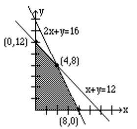
The shaded region where all conditions are satisfied is the feasible region or the feasible polygon.

The Fundamental Theorem of Linear Programming states that the maximum (or minimum) value of the objective function always takes place at the vertices of the feasible region.

Therefore, we will identify all the vertices (corner points) of the feasible region. These are found using any methods from Chapter 3 as we are looking for the points where any two of the boundary lines intersect. They are listed as (0, 0), (0, 12), (4, 8), (8, 0). To maximize Niki's income, we will substitute these points in the objective function to see which point gives us the highest income per week. We list the results below.

Critical Points	Income
(0, 0)	40(0) + 30(0) = $0
(0, 12)	40(0) + 30(12) = $360
(4, 8)	40(4) + 30(8) = $400
(8, 0)	40(8) + 30(0) = $320

Clearly, the point (4, 8) gives the most profit: $400.

Therefore, we conclude that Niki should work 4 hours at Job I, and 8 hours at Job II.

Example \(\PageIndex{2}\)

A factory manufactures two types of gadgets, regular and premium. Each gadget requires the use of two operations, assembly and finishing, and there are at most 12 hours available for each operation. A regular gadget requires 1 hour of assembly and 2 hours of finishing, while a premium gadget needs 2 hours of assembly and 1 hour of finishing. Due to other restrictions, the company can make at most 7 gadgets a day. If a profit of $20 is realized for each regular gadget and $30 for a premium gadget, how many of each should be manufactured to maximize profit?

Solution

We define our unknowns:

• Let the number of regular gadgets manufactured each day = \(x\).
• and the number of premium gadgets manufactured each day = \(y\).

The objective function is

\[P = 20x + 30y \nonumber\]

We now write the constraints. The fourth sentence states that the company can make at most 7 gadgets a day. This translates as

\[x + y \leq 7 \nonumber\]

Since the regular gadget requires one hour of assembly and the premium gadget requires two hours of assembly, and there are at most 12 hours available for this operation, we get

\[x + 2y \leq 12 \nonumber\]

Similarly, the regular gadget requires two hours of finishing and the premium gadget one hour. Again, there are at most 12 hours available for finishing. This gives us the following constraint.

\[2x + y \leq 12 \nonumber \]

The fact that \(x\) and \(y\) can never be negative is represented by the following two constraints:

\[x \geq 0 \text{, and } y \geq 0 \nonumber.\]

We have formulated the problem as follows:

\[\begin{array}{ll}
\textbf { Maximize } & \mathrm{P}=20 \mathrm{x}+30 \mathrm{y} \\
\textbf { Subject to: } & \mathrm{x}+\mathrm{y} \leq 7 \\
& \mathrm{x}+2\mathrm{y} \leq 12 \\
& 2\mathrm{x} +\mathrm{y} \leq 12 \\
& \mathrm{x} \geq 0 ; \mathrm{y} \geq 0
\end{array} \nonumber\]

In order to solve the problem, we next graph the constraints and feasible region.

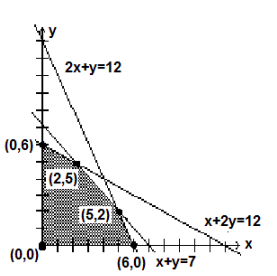
Again, we have shaded the feasible region, where all constraints are satisfied.

Since the extreme value of the objective function always takes place at the vertices of the feasible region, we identify all the critical points. They are listed as (0, 0), (0, 6), (2, 5), (5, 2), and (6, 0). To maximize profit, we will substitute these points in the objective function to see which point gives us the maximum profit each day. The results are listed below.

Critical Point	Income
(0, 0)	20(0) + 30(0) = $0
(0, 6)	20(0) + 30(6) = $180
(2, 5)	20(2) + 30(5) = $190
(5, 2)	20(5) + 30(2) = $160
(6,0)	20(6) + 30(0) = $120

The point (2, 5) gives the most profit, and that profit is $190.
Therefore, we conclude that we should manufacture 2 regular gadgets and 5 premium gadgets daily to obtain the maximum profit of $190.

So far we have focused on “standard maximization problems” in which

1. The objective function is to be maximized
2. All constraints are of the form \(ax + by \leq c\)
3. All variables are constrained to by non-negative (\(x ≥ 0\), \(y ≥ 0\))

We will next consider an example where that is not the case. Our next problem is said to have “mixed constraints”, since some of the inequality constraints are of the form \(ax + by ≤ c\) and some are of the form \(ax + by ≥ c\). The non-negativity constraints are still an important requirement in any linear program.

Example \(\PageIndex{3}\)

Solve the following maximization problem graphically.

\[\begin{array}{ll}
\textbf { Maximize } & \mathrm{P}=10 \mathrm{x}+15 \mathrm{y} \\
\textbf { Subject to: } & \mathrm{x}+\mathrm{y} \geq 1 \\
& \mathrm{x}+2\mathrm{y} \leq 6 \\
& 2\mathrm{x} +\mathrm{y} \leq 6 \\
& \mathrm{x} \geq 0 ; \mathrm{y} \geq 0
\end{array} \nonumber\]

Solution

The graph is shown below.

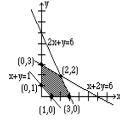
The five critical points are listed in the above figure. The reader should observe that the first constraint \(x + y ≥ 1\) requires that the feasible region must be bounded below by the line \(x + y =1\); the test point (0,0) does not satisfy \(x + y ≥ 1\), so we shade the region on the opposite side of the line from test point (0,0).

Critical point	Income
(1, 0)	10(1) + 15(0) = $10
(3, 0)	10(3) + 15(0) = $30
(2, 2)	10(2) + 15(2) = $50
(0, 3)	10(0) + 15(3) = $45
(0,1)	10(0) + 15(1) = $15

Clearly, the point (2, 2) maximizes the objective function to a maximum value of 50.

It is important to observe that that if the point (0,0) lies on the line for a constraint, then (0,0) could not be used as a test point. We would need to select any other point we want that does not lie on the line to use as a test point in that situation.

Finally, we address an important question. Is it possible to determine the point that gives the maximum value without calculating the value at each critical point?

The answer is yes.

We summarize:

The Maximization Linear Programming Problems

1. Define the unknowns.
2. Write the objective function that needs to be maximized.
3. Write the constraints.
   1. For the standard maximization linear programming problems, constraints are of the form: \(ax + by ≤ c\)
   2. Since the variables are non-negative, we include the constraints: \(x ≥ 0\); \(y ≥ 0\).
4. Graph the constraints.
5. Shade the feasible region.
6. Find the corner points.
7. Find the value of the objective function at each corner point to determine the corner point that gives the maximum value.