4.4: Linear Programming - Minimization Applications

Learning Objectives

In this section, you will learn to:

• Formulate minimization linear programming problems.
• Graph feasible regions for minimization linear programming problems.
• Determine optimal solutions for minimization linear programming problems.

Prerequisite Skills

Before you get started, take this prerequisite quiz.

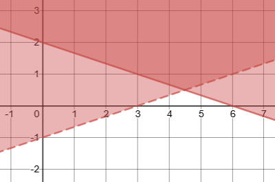
1. Graph this system of inequalities:

\(\left\{\begin{array} {l} x+3y\geq6\\y>\dfrac{1}{3}x-1\end{array}\right.\)

Click here to check your answer

If you missed this problem, review Section 4.2. (Note that this will open a different textbook in a new window.)

 

2. Graph this system of inequalities:

\(\left\{\begin{array} {l} y\geq 2x+1\\y\geq-3x+6\\x\geq0\\y\geq0\end{array}\right.\)

Click here to check your answer

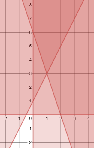
(The solution is in the upper center region.)

If you missed this problem, review Section 4.2. (Note that this will open a different textbook in a new window.)

Minimization linear programming problems are solved in much the same way as the maximization problems.

For the standard minimization linear program, the constraints are of the form \(ax + by ≥ c\), as opposed to the form \(ax + by ≤ c\) for the standard maximization problem. As a result, the feasible solution extends indefinitely to the upper right of the first quadrant, and is unbounded. But that is not a concern, since in order to minimize the objective function, the line associated with the objective function is moved towards the origin, and the critical point that minimizes the function is closest to the origin.

However, one should be aware that in the case of an unbounded feasible region, the possibility of no optimal solution exists.

Minimization Linear Programming Problems

1. Define the unknowns.
2. Write the objective function that needs to be minimized.
3. Write the constraints.
   1. For standard minimization linear programming problems, constraints are of the form: \(ax + by ≥ c\)
   2. Since the variables are non-negative, include the constraints: \(x ≥ 0\); \(y ≥ 0\).
4. Graph the constraints.
5. Shade the feasible region.
6. Find the corner points.
7. Find the value of the objective function at each corner point to determine the corner point that gives the minimum value.

Example \(\PageIndex{1}\)

At a university, Professor Symons wishes to employ two people, John and Mary, to grade papers for his classes. John is a graduate student and can grade 20 papers per hour; John earns $15 per hour for grading papers. Mary is a post-doctoral associate and can grade 30 papers per hour; Mary earns $25 per hour for grading papers. Each must be employed at least one hour a week to justify their employment.

If Prof. Symons has at least 110 papers to be graded each week, how many hours per week should he employ each person to minimize the cost?

Solution

We define the unknowns as follows:

Let the number of hours per week John is employed = \(x\).

and the number of hours per week Mary is employed = \(y\).

The objective function is

\[C = 15x + 25y \nonumber \]

The fact that each must work at least one hour each week results in the following two constraints:

\[\begin{array}{l}
x \geq 1 \\
y \geq 1
\end{array} \nonumber \]

Since John can grade 20 papers per hour and Mary 30 papers per hour, and there are at least 110 papers to be graded per week, we get

\[20x + 30y ≥ 110 \nonumber\]

The fact that \(x\) and \(y\) are non-negative, we get

\[x ≥ 0 \text{, and } y ≥ 0. \nonumber\]

The problem has been formulated as follows.

\[\begin{array}{ll}
\textbf { Minimize } & \mathrm{C}=15 \mathrm{x}+25 \mathrm{y} \\
\textbf { Subject to: } & \mathrm{x} \geq 1 \\
& \mathrm{y} \geq 1 \\
& 20 \mathrm{x}+30 \mathrm{y} \geq 110 \\
& \mathrm{x} \geq 0 ; \mathrm{y} \geq 0
\end{array} \nonumber\]

To solve the problem, we graph the constraints as follows:

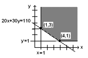
Again, we have shaded the feasible region, where all constraints are satisfied.

If we used test point (0,0) that does not lie on any of the constraints, we observe that (0, 0) does not satisfy any of the constraints \(x ≥ 1\), \(y ≥ 1\), \(20x + 30y ≥ 110\). Thus all the shading for the feasible region lies on the opposite side of the constraint lines from the point (0,0).

Alternatively we could use test point (4,6), which also does not lie on any of the constraint lines. We’d find that (4,6) does satisfy all of the inequality constraints. Consequently all the shading for the feasible region lies on the same side of the constraint lines as the point (4,6).

Since the extreme value of the objective function always takes place at the vertices of the feasible region, we identify the two critical points, (1, 3) and (4, 1). To minimize cost, we will substitute these points in the objective function to see which point gives us the minimum cost each week. The results are listed below.

Critical points	Income
(1, 3)	15(1) + 25(3) = $90
(4, 1)	15(4) + 25(1) = $85

The point (4, 1) gives the least cost, and that cost is $85. Therefore, we conclude that in order to minimize grading costs, Professor Symons should employ John 4 hours a week, and Mary 1 hour a week at a cost of $85 per week.

Example \(\PageIndex{2}\)

Professor Hamer is on a low cholesterol diet. During lunch at the college cafeteria, he always chooses between two meals: pasta or tofu. The table below lists the amount of protein, carbohydrates, and vitamins each meal provides along with the amount of cholesterol he is trying to minimize. Mr. Hamer needs at least 200 grams of protein, 960 grams of carbohydrates, and 40 grams of vitamins for lunch each month. Over this time period, how many days should he have the pasta meal, and how many days the tofu meal so that he gets the adequate amount of protein, carbohydrates, and vitamins and at the same time minimizes his cholesterol intake?

	PASTA	TOFU
PROTEIN	8g	16g
CARBOHYDRATES	60g	40g
VITAMIN C	2g	2g
CHOLESTEROL	60mg	50mg

Solution

We define the unknowns as follows.

Let the number of days Mr. Hamer eats pasta = \(x\).

and the number of days Mr. Hamer eats tofu = \(y\).

Since he is trying to minimize his cholesterol intake, our objective function represents the total amount of cholesterol C provided by both meals.

\[C = 60x + 50y \nonumber \]

The constraint associated with the total amount of protein provided by both meals is

\[8x + 16y ≥ 200 \nonumber \]

Similarly, the two constraints associated with the total amount of carbohydrates and vitamins are obtained, and they are

\[\begin{array}{l}
60 x+40 y \geq 960 \\
2 x+2 y \geq 40
\end{array} \nonumber\]

The constraints that state that x and y are non-negative are

\[x ≥ 0 \text{, and } y ≥ 0 \nonumber.\]

We summarize all information as follows:

\[\begin{array}{ll}
\textbf { Minimize } & \mathrm{C}=60 \mathrm{x}+50 \mathrm{y} \\
\textbf { Subject to: } & 8 \mathrm{x}+16 \mathrm{y} \geq 200 \\
& 60 \mathrm{x}+40 \mathrm{y} \geq 960 \\
& 2 \mathrm{x}+2 \mathrm{y} \geq 40 \\
& \mathrm{x} \geq 0 ; \mathrm{y} \geq 0
\end{array} \nonumber\]

To solve the problem, we graph the constraints and shade the feasible region.

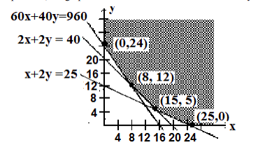
We have shaded the unbounded feasible region, where all constraints are satisfied.

To minimize the objective function, we find the vertices of the feasible region. These vertices are (0, 24), (8, 12), (15, 5) and (25, 0). To minimize cholesterol, we will substitute these points in the objective function to see which point gives us the smallest value. The results are listed below.

Critical points	Income
(0, 24)	60(0) + 50(24) = 1200
(8, 12)	60(8) + 50(12) = 1080
(15, 5)	60(15) + 50(5) = 1150
(25, 0)	60(25) + 50(0) = 1500

The point (8, 12) gives the least cholesterol, which is 1080 mg. This states that for every 20 meals, Professor Hamer should eat pasta 8 days, and tofu 12 days.

We must be aware that in some cases, a linear program may not have an optimal solution.

• A linear program can fail to have an optimal solution is if there is not a feasible region. If the inequality constraints are not compatible, there may not be a region in the graph that satisfies all the constraints. If the linear program does not have a feasible solution satisfying all constraints, then it can not have an optimal solution.
• A linear program can fail to have an optimal solution if the feasible region is unbounded.
  • The two minimization linear programs we examined had unbounded feasible regions. The feasible region was bounded by constraints on some sides but was not entirely enclosed by the constraints. Both of the minimization problems had optimal solutions.
  • However, if we were to consider a maximization problem with a similar unbounded feasible region, the linear program would have no optimal solution. No matter what values of x and y were selected, we could always find other values of \(x\) and \(y\) that would produce a higher value for the objective function. In other words, if the value of the objective function can be increased without bound in a linear program with an unbounded feasible region, there is no optimal maximum solution.

Although the method of solving minimization problems is similar to that of the maximization problems, we still feel that we should summarize the steps involved.

Minimization Linear Programming Problems

1. Define the unknowns.
2. Write the objective function that needs to be minimized.
3. Write the constraints.
   1. For standard minimization linear programming problems, constraints are of the form: \(ax + by ≥ c\)
   2. Since the variables are non-negative, include the constraints: \(x ≥ 0\); \(y ≥ 0\).
4. Graph the constraints.
5. Shade the feasible region.
6. Find the corner points.
7. Find the value of the objective function at each corner point to determine the corner point that gives the minimum value.