
1.6: Graphs of Functions


- Last updated
- Sep 2, 2024
- Save as PDF

( \newcommand{\kernel}{\mathrm{null}\,}\)
The following topics related to the material in this section are assumed prerequisites for this course. They are only covered if you are enrolled in a class with corequisite support:
- Factoring trinomials
Topics that must be assumed prerequisites (even for a class with corequisite support) are:
- Using the Zero Factor Property to solve polynomial equations
- Use the Fundamental Graphing Principle for Functions to graph a function by point-plotting.
- Graph a piecewise function using point-plotting.
- Identify the zeros of a function from its graph.
- Determine if a function is odd, even, or neither.
- Use graphing technology to graph a function.
- Identify the interval(s) over which the graph of a function is increasing, decreasing, or constant.
- Given the graph of a function (or given a function that can easily be graphed), state local and absolute extrema.
- Use graphing technology to approximate local and absolute extrema (along with intervals of increase, decrease, and constancy).
Graphing Functions by Point-Plotting
In Section 1.3, we defined a function as a special type of relation; one in which each x-coordinate was matched with only one y-coordinate. We spent most of our time in that section looking at functions graphically because they were, after all, just sets of points in the plane. Then, in Section 1.4, we described a function as a process and defined the notation necessary to work with functions algebraically. So now it’s time to look at functions graphically again, only this time we’ll do so with the notation defined in Section 1.4. We start with what should not be a surprising connection.
The graph of a function f is the set of points which satisfy the equation y=f(x). That is, the point (x,y) is on the graph of f if and only if y=f(x).
Graph f(x)=x2−x−6.
- Solution
-
To graph f, we graph the equation y=f(x). To this end, we use the techniques outlined previously. Specifically, we check for intercepts, test for symmetry, and plot additional points as needed. To find the x-intercepts, we set y=0. Since y=f(x), this means f(x)=0.f(x)=x2−x−6⟹0=x2−x−6⟹0=(x−3)(x+2)This implies either x−3=0 or x+2=0. Therefore, x=3 or x=−2. So we get (−2,0) and (3,0) as x-intercepts. To find the y-intercept, we set x=0. Using function notation, this is the same as finding f(0) and f(0)=02−0−6=−6. Thus the y-intercept is (0,−6).
As far as symmetry is concerned, we can tell from the intercepts that the graph possesses none of the three symmetries discussed thus far.1 We can make a table analogous to the ones we made in Section 1.2, plot the points and connect the dots in a somewhat pleasing fashion to get the graph below.

As has been mentioned previously, graphing a function (or relation) by making a table of values and plotting points is only an acceptable method of graphing while we are in the beginning of learning College Algebra. In your Algebra course(s), you learned to graph functions via transformations. This is the method we will review in Section 1.7 and it is the only method you will use to graph from that point forward.
We can see that graphing simple quadratic functions is not too bad, but graphing piecewise-defined functions is a bit more of a challenge.
Graph the following (piecewise) function.f(x)={4−x2 if x<1x−3, if x≥1
- Solution
-
We proceed as before – finding intercepts, testing for symmetry and then plotting additional points as needed.
To find the x-intercepts, as before, we set f(x)=0. The twist is that we have two formulas for f(x). For x<1, we use the formula f(x)=4−x2. Setting f(x)=0 gives 0=4−x2, so that x=±2. However, of these two answers, only x=−2 fits in the domain x<1 for this piece. This means the only x-intercept for the x<1 region of the x-axis is (−2,0). For x≥1, f(x)=x−3. Setting f(x)=0 gives 0=x−3, or x=3. Since x=3 satisfies the inequality x≥1, we get (3,0) as another x-intercept.
Next, we seek the y-intercept. Notice that x=0 falls in the domain x<1. Thus f(0)=4−02=4 yields the y-intercept (0,4).
As far as symmetry is concerned, you can check that the equation y=4−x2 is symmetric about the y-axis; unfortunately, this equation (and its symmetry) is valid only for x<1. You can also verify y=x−3 possesses none of the symmetries discussed in the Section 1.2.
When plotting additional points, it is important to keep in mind the restrictions on x for each piece of the function. The sticking point for this function is x=1, since this is where the equations change. When x=1, we use the formula f(x)=x−3, so the point on the graph (1,f(1)) is (1,−2). However, for all values less than 1, we use the formula f(x)=4−x2. Thus for the values x=0.9, x=0.99, x=0.999, and so on, we find the corresponding y-values using the formula f(x)=4−x2. Making a table as before, we see that as the x values sneak up to x=1 in this fashion, the f(x) values inch closer and closer to 4−12=3. To indicate this graphically, we use an open circle at the point (1,3).
Putting all of this information together and plotting additional points, we get

In the previous two examples, the x-coordinates of the x-intercepts of the graph of y=f(x) were found by solving f(x)=0. For this reason, they are called the zeros of f.
The zeros of a function f are the solutions to the equation f(x)=0.
In other words, x is a zero of f if and only if (x,0) is an x-intercept of the graph of y=f(x).
Symmetry of Graphs of Functions
Of the three symmetries discussed in Section 1.2, only two are of significance to functions: symmetry about the y-axis and symmetry about the origin.2 Recall that we can test whether the graph of an equation is symmetric about the y-axis by replacing x with −x and checking to see if an equivalent equation results. If we are graphing the equation y=f(x), substituting −x for x results in the equation y=f(−x). In order for this equation to be equivalent to the original equation y=f(x), we need f(−x)=f(x).
In a similar fashion, we recall that to test an equation’s graph for symmetry about the origin, we replace x and y with −x and −y, respectively. Doing this substitution in the equation y=f(x) results in −y=f(−x). Solving the latter equation for y gives y=−f(−x). In order for this equation to be equivalent to the original equation y=f(x) we need −f(−x)=f(x), or, equivalently, f(−x)=−f(x).
The graph of a function f is symmetric
- about the y-axis if and only if f(−x)=f(x) for all x in the domain of f.
- about the origin if and only if f(−x)=−f(x) for all x in the domain of f.
For reasons which won’t become clear until we study polynomials, we call a function even if its graph is symmetric about the y-axis or odd if its graph is symmetric about the origin. Apart from a very specialized family of functions which are both even and odd, functions fall into one of three distinct categories: even, odd, or neither even nor odd.
Determine, analytically,3 if the following functions are even, odd, or neither even nor odd. Verify your result with graphing technology.
- f(x)=52−x2
- g(x)=5x2−x2
- h(x)=5x2−x3
- i(x)=5x2x−x3
- j(x)=x2−x100−1
- p(x)={x+3 if x<0−x+3, if x≥0
- Solutions
-
The first step in all of these problems is to replace x with −x and simplify.
- Given f(x)=52−x2,f(−x)=52−(−x)2=52−x2=f(x)Hence, f is even. Desmos furnishes the following.
This suggests that the graph of f is symmetric about the y-axis, as expected.
- Given g(x)=5x2−x2, g(−x)=5(−x)2−(−x)2=−5x2−x2It doesn’t appear that g(−x) is equivalent to g(x). To prove this, we check with an x-value. After some trial and error, we see that g(1)=5 whereas g(−1)=−5. This proves that g is not even, but it doesn’t rule out the possibility that g is odd. (Why not?) To check if g is odd, we compare g(−x) with −g(x)−g(x)=−5x2−x2=−5x2−x2=g(−x)Hence, g is odd. Graphically,
Desmos indicates the graph of g is symmetric about the origin, as expected.
- Given h(x)=5x2−x3,h(−x)=5(−x)2−(−x)3=−5x2+x3Once again, h(−x) doesn’t appear to be equivalent to h(x). We check with an x value, for example, h(1)=5 but h(−1)=−53. This proves that h is not even and it also shows h is not odd. (Why?) Graphically,
The graph of h appears to be neither symmetric about the y-axis nor the origin.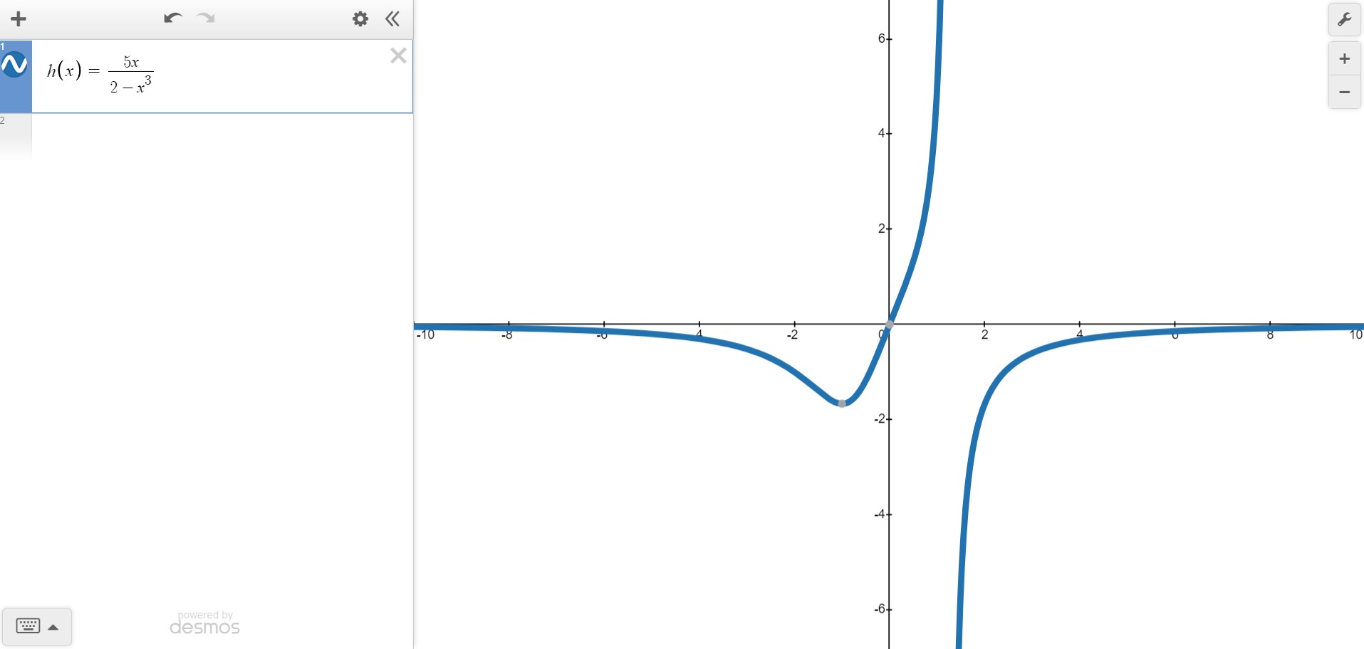
- Given i(x)=5x2x−x3, i(−x)=5(−x)2(−x)−(−x)3=−5x−2x+x3The expression i(−x) doesn’t appear to be equivalent to i(x). However, after checking some x values, for example x=1 yields i(1)=5 and i(−1)=5, it appears that i(−x) does, in fact, equal i(x). However, while this suggests i is even, it doesn’t prove it. (It does, however, prove i is not odd.)
To prove i(−x)=i(x), we need to manipulate our expressions for i(x) and i(−x) and show that they are equivalent. A clue as to how to proceed is in the numerators: in the formula for i(x), the numerator is 5x and in i(−x) the numerator is −5x. To re-write i(x) with a numerator of −5x, we need to multiply its numerator by −1. To keep the value of the fraction the same, we need to multiply the denominator by −1 as well. Thusi(x)=5x2x−x3=(−1)5x(−1)(2x−x3)=−5x−2x+x3=i(−x)Hence, i is even. Desmos supports our conclusion.
- Given j(x)=x2−x100−1, j(−x)=(−x)2−−x100−1=x2+x100−1The expression for j(−x) doesn’t seem to be equivalent to j(x), so we check using x=1 to get j(1)=−1100 and j(−1)=1100. This rules out j being even. However, it doesn’t rule out j being odd. Examining −j(x) gives−j(x)=−(x2−x100−1)=−x2+x100+1The expression −j(x) doesn’t seem to match j(−x) either. Testing x=2 gives j(2)=14950 and j(−2)=15150, so j is not odd, either. Desmos gives the following:
Desmos suggests that the graph of j is symmetric about the y-axis which would imply that j is even. However, we have proven that is not the case. This is a great example that technology can fail us!
- Testing the graph of y=p(x) for symmetry is complicated by the fact p(x) is a piecewise defined function. As always, we handle this by checking the condition for symmetry by checking it on each piece of the domain.
We first consider the case when x<0 and set about finding the correct expression for p(−x). Even though p(x)=x+3 for x<0, p(−x)≠−x+3 here. The reason for this is that since x<0, −x>0 which means to find p(−x), we need to use the other formula for p(x), namely p(x)=−x+3. Hence, for x<0, p(−x)=−(−x)+3=x+3=p(x).
For x≥0, p(x)=−x+3 and we have two cases. If x>0, then −x<0 so p(−x)=(−x)+3=−x+3=p(x). If x=0, then p(0)=3=p(−0). Hence, in all cases, p(−x)=p(x), so p is even. Since p(0)=3 but p(−0)=p(0)=3≠−3, we also have p is not odd.
While graphing y=p(x) is not onerous to do by hand, it is instructive to see how to enter this into Desmos. By using some of the logical commands (see how I entered the commands in the figure below), we have:
Desmos shows that the graph appears to be symmetric about the y-axis.
- Given f(x)=52−x2,f(−x)=52−(−x)2=52−x2=f(x)Hence, f is even. Desmos furnishes the following.
There are two lessons to be learned from the last example. The first is that sampling function values at particular x values is not enough to prove that a function is even or odd − despite the fact that j(−1)=−j(1), j turned out not to be odd. Secondly, while Desmos (and your graphing calculator) may suggest mathematical truths, it is the Algebra which proves mathematical truths.
Increasing, Decreasing, and Constant Behavior
We now wish to address general function behavior. As you shall see in the next several chapters, each family of functions has its own unique attributes and we will study them all in great detail. The purpose of this section’s discussion, then, is to lay the foundation for that further study by investigating aspects of function behavior which apply to all functions. To start, we will examine the concepts of when a function is increasing, decreasing, and constant. Before defining the concepts algebraically, it is instructive to look at them graphically. Consider Figure 1.6.1, which is the graph of the function f.

Figure 1.6.1
Reading from left-to-right, the graph "starts" at the point (−4,−3) and "ends" at the point (6,5.5). If we imagine walking from left-to-right on the graph, between (−4,−3) and (−2,4.5), we are walking "uphill"; then between (−2,4.5) and (3,−8), we are walking "downhill"; and between (3,−8) and (4,−6), we are walking "uphill" once more. From (4,−6) to (5,−6), we "level off", and then resume walking "uphill" from (5,−6) to (6,5.5).
In other words, for the x-values between −4 and −2, the y-coordinates on the graph are getting larger, or increasing, as we move from left-to-right. Since y=f(x), the y-values on the graph are the function values, and we say that the function f is increasing on the interval (−4,−2). Analogously, we say that f is decreasing on the interval (−2,3), increasing once more on the interval (3,4), constant on (4,5), and finally increasing once again on (5,6).
It is extremely important to notice that the behavior (increasing, decreasing or constant) occurs on an open interval consisting of x values. When we say that the function f is increasing on (−4,−2), we do not mention the actual y values that f attains along the way. Thus, we report where the behavior occurs, not to what extent the behavior occurs.
Also, as a convention, we do not include the endpoints of the interval over which a function is increasing, decreasing, or constant.4 This is because a function technically cannot be increasing or decreasing at a specific point. We can see why in Figure 1.6.1. x=−2 is contained in an interval on which f is increasing and one on which it is decreasing. So would it be correct to say that f is increasing on [−4,−2] and decreasing on [−2,3]? I would hope you see the issue - if we said this, then we are saying that f is increasing at x=−2 and decreasing at x=−2.
We’re now ready for the more formal algebraic definitions of what it means for a function to be increasing, decreasing or constant.
Suppose f is a function defined on an open interval I. We say f is:
- increasing on I if and only if f(a)<f(b) for all real numbers a, b in I with a<b.
- decreasing on I if and only if f(a)>f(b) for all real numbers a, b in I with a<b.
- constant on I if and only if f(a)=f(b) for all real numbers a, b in I.
It is worth taking some time to see that the algebraic descriptions of increasing, decreasing and constant as stated in this definition agree with our graphical descriptions given earlier. You should look back through the examples and exercise sets in previous sections where graphs were given to see if you can determine the intervals on which the functions are increasing, decreasing or constant. Can you find an example of a function for which none of the concepts in this definition apply?
Local and Absolute Extrema
Now let’s turn our attention to a few of the points on the graph in Figure 1.6.1. Clearly the point (−2,4.5) does not have the largest y-value of all of the points on the graph of f − indeed that honor goes to (6,5.5) − but (−2,4.5) should get some sort of consolation prize for being "the top of the hill" between x=−4 and x=3.
We say that the function f has a local maximum (also known as a relative maximum) at the point (−2,4.5), because the y-coordinate, 4.5, is the largest y-value (hence, function value) on the curve "near" x=−2. Similarly, we say that the function f has a local minimum (also known as a relative minimum) at the point (3,−8), since the y-coordinate, −8, is the smallest function value near x=3.
A local maximum or local minimum is also referred to as a local extremum. The plural of extremum is extrema. Therefore, if you are talking about a group of local maximums and/or minimums, you would call them local extrema.
Although it is tempting to say that local extrema occur when the function changes from increasing to decreasing or vice versa, this "definition" is not precise enough for the needs of Calculus. At the risk of being pedantic, we will present the traditional definitions and thoroughly vet the pathologies they induce in the Exercises. We have one last observation to make before we proceed to the algebraic definitions and look at a fairly tame, yet helpful, example.
If we look at the entire graph, we see that the largest y value (the largest function value) is 5.5 at x=6. In this case, we say the absolute maximum (also called the global maximum, or simply the maximum) of f is 5.5; similarly, the absolute minimum (again, also called the global minimum, or simply the minimum) of f is −8.
We formalize these concepts in the following definitions.
Suppose f is a function with f(a)=b.
- We say f has a local maximum at the point (a,b) if and only if there is an open interval I containing a for which f(a)≥f(x) for all x in I. The value f(a)=b is called a local maximum value of f in this case.
- We say f has a local minimum at the point (a,b) if and only if there is an open interval I containing a for which f(a)≤f(x) for all x in I. The value f(a)=b is called a local minimum value of f in this case.
- The value b is called the absolute maximum of f if b≥f(x) for all x in the domain of f.
- The value b is called the absolute minimum of f if b≤f(x) for all x in the domain of f.
It’s important to note that not every function will have all of these features. Indeed, it is possible to have a function with no local or absolute extrema at all! (Any ideas of what such a function’s graph would have to look like?) We shall see examples of functions in the Exercises which have one or two, but not all, of these features, some that have instances of each type of extremum, and some functions that seem to defy common sense. In all cases, though, we shall adhere to the algebraic definitions above as we explore the wonderful diversity of graphs that functions provide us.
Here is the "tame" example which was promised earlier. It summarizes all of the concepts presented in this section as well as some from previous sections so you should spend some time thinking deeply about it before proceeding to the Exercises.
Given the graph of y=f(x), answer all of the following questions.

- Find the domain of f.
- Find the range of f.
- List the x-intercepts, if any exist.
- List the y-intercepts, if any exist.
- Find the zeros of f.
- Solve f(x)<0.
- Determine f(2).
- Solve f(x)=−3.
- Find the number of solutions to f(x)=1.
- Does f appear to be even, odd, or neither?
- List the intervals on which f is increasing.
- List the intervals on which f is decreasing.
- List the local maximums, if any exist.
- List the local minimums, if any exist.
- Find the maximum, if it exists.
- Find the minimum, if it exists.
- Solutions
-
- To find the domain of f, we proceed as in Section 1.3. By projecting the graph to the x-axis, we see that the portion of the x-axis which corresponds to a point on the graph is everything from −4 to 4, inclusive. Hence, the domain is [−4,4].
- To find the range, we project the graph to the y-axis. We see that the y-values from −3 to 3, inclusive, constitute the range of f. Hence, our answer is [−3,3].
- The x-intercepts are the points on the graph with y-coordinate 0, namely (−2,0) and (2,0).
- The y-intercept is the point on the graph with x-coordinate 0, namely (0,3).
- The zeros of f are the x-coordinates of the x-intercepts of the graph of y=f(x) which are x=−2,2.
- To solve f(x)<0, we look for the x values of the points on the graph where the y-coordinate is less than 0. Graphically, we are looking for where the graph is below the x-axis. This happens for the x values from −4 to −2 and again from 2 to 4. So our answer is [−4,−2)∪(2,4]. It is important to understand why we did not include ±2 in those intervals.
- Since the graph of f is the graph of the equation y=f(x), f(2) is the y-coordinate of the point which corresponds to x=2. Since the point (2,0) is on the graph, we have f(2)=0.
- To solve f(x)=−3, we look where y=f(x)=−3. We find two points with a y-coordinate of −3, namely (−4,−3) and (4,−3). Hence, the solutions to f(x)=−3 are x=±4.
- As in the previous problem, to solve f(x)=1, we look for points on the graph where the y-coordinate is 1. Even though these points aren’t specified, we see that the curve has two points with a y-value of 1, as seen in the figure below. That means there are two solutions to f(x)=1.
The graph appears to be symmetric about the y-axis. This suggests (but does not prove) that f is even.
- As we move from left-to-right, the graph rises from the point (−4,−3) to the point (0,3). This means f is increasing on the interval (of x values) (−4,0). (Remember, the answer here is an open interval on the x-axis.)
- As we move from left-to-right, the graph falls from the point (0,3) to the point (4,−3). This means f is decreasing on the interval (0,4). (Remember, the answer here is an open interval on the x-axis.)
- The function has its only local maximum at (0,3), so f(0)=3 is the local maximum value.
- There are no local minimums. Why don’t (−4,−3) and (4,−3) count?
Let’s consider the point (−4,−3) for a moment. Recall that, in the definition of local minimum, there needs to be an open interval I which contains x=−4 such that f(−4)<f(x) for all x in I different from −4. But if we put an open interval around x=−4 a portion of that interval will lie outside of the domain of f. Because we are unable to fulfill the requirements of the definition for a local minimum, we cannot claim that f has one at (−4,−3). The point (4,−3) fails for the same reason − no open interval around x=4 stays within the domain of f. - The maximum value of f is the largest y-coordinate which is 3.
- The minimum value of f is the smallest y-coordinate which is −3.
Using Graphing Technology for Approximations
With few exceptions, we will not develop techniques in College Algebra which allow us to determine the intervals on which a function is increasing, decreasing, or constant, or to find the local maximums and local minimums analytically; this is the business of Calculus. When we have need to find such beasts, we will resort to graphing technology. Most graphing technologies have "Minimum" and "Maximum" features which can be used to approximate these values, as we now demonstrate using Desmos.
Let f(x)=15xx2+3. Use Desmos to approximate the intervals on which f is increasing and those on which it is decreasing. Approximate all extrema.
- Solution
-
Entering this function into Desmos gives the following:

All we need to do is click anywhere on the graphed curve and Desmos immediately plots points for the extrema and the intercept(s). Clicking on those points, Desmos will give approximations to the x- and y-values (unfortunately, only to a maximum of three decimal places).

Therefore, to three decimal places, f appears to have its only local minimum at the point (−1.732,−4.33) and its only local maximum at the point (1.732,4.33). Given the symmetry about the origin suggested by the graph (again, not a proof), the relation between these points shouldn’t be too surprising. The function appears to be increasing on the interval (−1.732,1.732) and decreasing on the interval (−∞,−1.732)∪(1.732,∞). This makes −4.33 the (absolute) minimum and 4.33 the (absolute) maximum.
Our final example is borrowed from Calculus. Since we do not have the mathematical tools at this time to do this any other way, we resort to technology.
Find the points on the graph of y=(x−3)2 which are closest to the origin. Round your answers to two decimal places.
- Solution
-
Suppose a point (x,y) is on the graph of y=(x−3)2. Its distance to the origin (0, 0) is given byd=√(x−0)2+(y−0)2=√x2+y2=√x2+[(x−3)2]2(substituting)=√x2+(x−3)4Given a value for x, the formula d=√x2+(x−3)4 is the distance from (0,0) to the point (x,y) on the curve y=(x−3)2. What we have defined, then, is a function d(x) which we wish to minimize over all values of x. To accomplish this task analytically would require Calculus. Since we are not quite in Calculus yet, we can use graphing technology to find an approximate solution. Using Desmos, we enter the function d(x) as shown in Figure 1.6.4.

Figure 1.6.4The solid curve represents the distances from the graph of y=(x−3)2 (the dashed curve) to the origin. We see that the (absolute) minimum occurs near x=2 (we cannot be certain that this is exact until we reach Calculus). To find the y value on the parabola associated with x=2, we substitute 2 into the equation to get y=(x−3)2=(2−3)2=1. So, our final answer is (2,1).
It's important to note that any result garnered from a calculator in this fashion is an approximation, and should be treated as such. (What does the y-value of 2.236 in Figure 1.6.4 mean in this problem?)
Footnotes
1 You should verify this.
2 Why do you think we don't concern ourselves with symmetry about the x-axis when speaking of functions?
3 "Analytically" means "by hand."
4 It's an unfortunate reality that some authors (and instructors) don't understand the issue with including endpoints on intervals of increase, decrease, or constancy.