1.6E: Exercises

Exercises

In Exercises 1 - 12, sketch the graph of the given function via building a table of values and point-plotting (for now). State the domain of the function, identify any intercepts and test for symmetry.

1. \(\ f(x) = 2 − x\)
2. \(\ f(x)=\frac{x-2}{3}\)
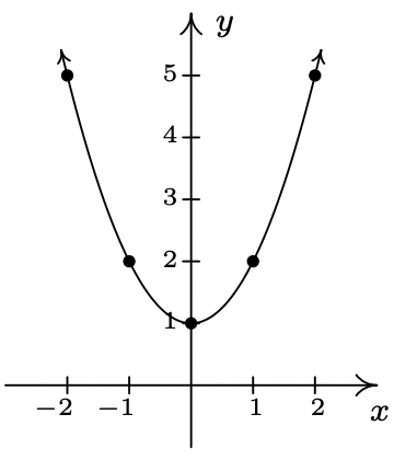
3. \(\ f(x)=x^{2}+1\)
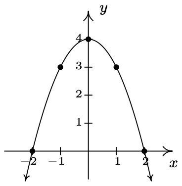
4. \(\ f(x)=4-x^{2}\)
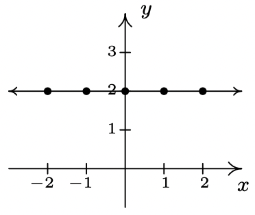
5. \(\ f(x) = 2\)
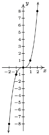
6. \(\ f(x)=x^{3}\)
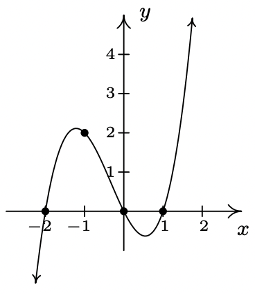
7. \(\ f(x) = x(x − 1)(x + 2)\)
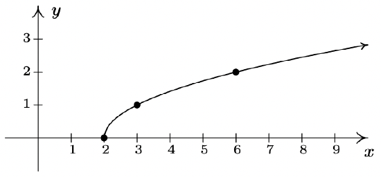
8. \(\ f(x)=\sqrt{x-2}\)
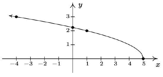
9. \(\ f(x)=\sqrt{5-x}\)
10. \(\ f(x)=3-2 \sqrt{x+2}\)
11. \(\ f(x)=\sqrt[3]{x}\)
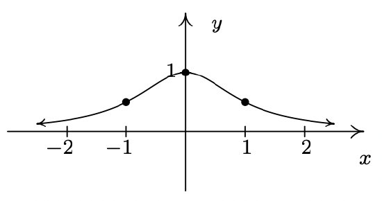
12. \(\ f(x)=\frac{1}{x^{2}+1}\)

In Exercises 13 - 20, sketch the graph of the given piecewise-defined function via building a table of values and point-plotting (for now).

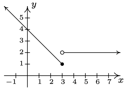
13. \(\ f(x)=\left\{\begin{array}{rlr}
    4-x & \text { if } & x \leq 3 \\
    2 & \text { if } & x>3
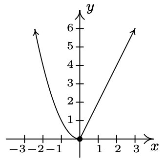
    \end{array}\right.\)
14. \(\ f(x)=\left\{\begin{array}{lll}
    x^{2} & \text { if } & x \leq 0 \\
    2 x & \text { if } & x>0
    \end{array}\right.\)
15. \(\ f(x)=\left\{\begin{array}{rll}
    -3 & \text { if } & x<0 \\
    2 x-3 & \text { if } & 0 \leq x \leq 3 \\
    3 & \text { if } & x>3
    \end{array}\right.\)
16. \(\ f(x)=\left\{\begin{array}{lll}
    x^{2}-4 & \text { if } & x \leq-2 \\
    4-x^{2} & \text { if } & -2<x<2 \\
    x^{2}-4 & \text { if } & x \geq 2
    \end{array}\right.\)
17. \(\ f(x)=\left\{\begin{array}{rll}
    -2 x-4 & \text { if } & x<0 \\
    3 x & \text { if } & x \geq 0
    \end{array}\right.\)
18. \(\ f(x)=\left\{\begin{array}{lll}
    \sqrt{x+4} & \text { if } & -4 \leq x<5 \\
    \sqrt{x-1} & \text { if } & x \geq 5
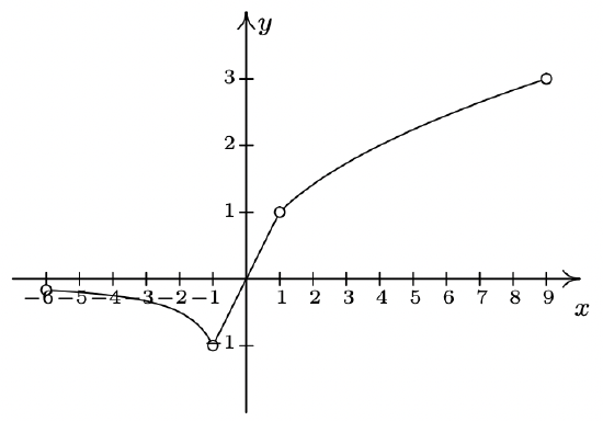
    \end{array}\right.\)
19. \(\ f(x)=\left\{\begin{array}{rll}
    x^{2} & \text { if } & x \leq-2 \\
    3-x & \text { if } & -2<x<2 \\
    4 & \text { if } & x \geq 2
    \end{array}\right.\)
20. \(\ f(x)=\left\{\begin{array}{rll}
    \frac{1}{x} & \text { if } & -6<x<-1 \\
    x & \text { if } & -1<x<1 \\
    \sqrt{x} & \text { if } & 1<x<9
    \end{array}\right.\)

In Exercises 21 - 41, determine analytically if the following functions are even, odd or neither.

21. \(\ f(x) = 7x\)
22. \(\ f(x) = 7x + 2\)
23. \(\ f(x) = 7\)
24. \(\ f(x)=3 x^{2}-4\)
25. \(\ f(x)=4-x^{2}\)
26. \(\ f(x)=x^{2}-x-6\)
27. \(\ f(x)=2 x^{3}-x\)
28. \(\ f(x)=-x^{5}+2 x^{3}-x\)
29. \(\ f(x)=x^{6}-x^{4}+x^{2}+9\)
30. \(\ f(x)=x^{3}+x^{2}+x+1\)
31. \(\ f(x)=\sqrt{1-x}\)
32. \(\ f(x)=\sqrt{1-x^{2}}\)
33. \(\ f(x) = 0\)
34. \(\ f(x)=\sqrt[3]{x}\)
35. \(\ f(x)=\sqrt[3]{x^{2}}\)
36. \(\ f(x)=\frac{3}{x^{2}}\)
37. \(\ f(x)=\frac{2 x-1}{x+1}\)
38. \(\ f(x)=\frac{3 x}{x^{2}+1}\)
39. \(\ f(x)=\frac{x^{2}-3}{x-4 x^{3}}\)
40. \(\ f(x)=\frac{9}{\sqrt{4-x^{2}}}\)
41. \(\ f(x)=\frac{\sqrt[3]{x^{3}+x}}{5 x}\)

In Exercises 42 - 57, use the graph of \(\ y = f(x)\) given below to answer the question.

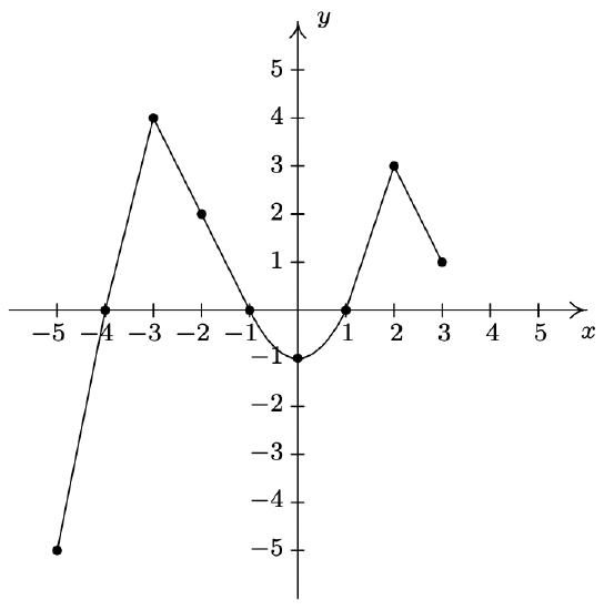
42. Find the domain of \(\ f\).
43. Find the range of \(\ f\).
44. Determine \(\ f(−2)\).
45. Solve \(\ f(x) = 4\).
46. List the x-intercepts, if any exist.
47. List the y-intercepts, if any exist.
48. Find the zeros of \(\ f\).
49. Solve \(\ f(x) ≥ 0\).
50. Find the number of solutions to \(\ f(x) = 1\).
51. Does \(\ f\) appear to be even, odd, or neither?
52. List the intervals where \(\ f\) is increasing.
53. List the intervals where \(\ f\) is decreasing.
54. List the local maximums, if any exist.
55. List the local minimums, if any exist.
56. Find the maximum, if it exists.
57. Find the minimum, if it exists.

In Exercises 58 - 73, use the graph of \(\ y = f(x)\) given below to answer the question.

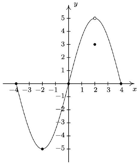
58. Find the domain of \(\ f\).
59. Find the range of \(\ f\).
60. Determine \(\ f(2)\).
61. Solve \(\ f(x) = −5\).
62. List the x-intercepts, if any exist.
63. List the y-intercepts, if any exist.
64. Find the zeros of \(\ f\).
65. Solve \(\ f(x) ≤ 0\).
66. Find the number of solutions to \(\ f(x) = 3\).
67. Does \(\ f\) appear to be even, odd, or neither?
68. List the intervals where \(\ f\) is increasing.
69. List the intervals where \(\ f\) is decreasing.
70. List the local maximums, if any exist.
71. List the local minimums, if any exist.
72. Find the maximum, if it exists.
73. Find the minimum, if it exists.

In Exercises 74 - 77, use graphing technology to approximate the local and absolute extrema of the given function. Approximate the intervals on which the function is increasing and those on which it is decreasing. Round your answers to two decimal places.

74. \(\ f(x)=x^{4}-3 x^{3}-24 x^{2}+28 x+48\)
75. \(\ f(x)=x^{2 / 3}(x-4)\)
76. \(\ f(x)=\sqrt{9-x^{2}}\)
77. \(\ f(x)=x \sqrt{9-x^{2}}\)

In Exercises 78 - 85, use the graphs of \(\ y = f(x)\) and \(\ y = g(x)\) below to find the function value.

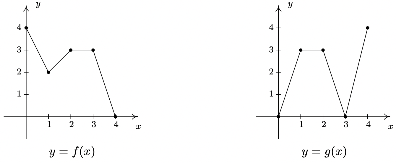
78. \(\ (f + g)(0)\)
79. \(\ (f + g)(1)\)
80. \(\ (f − g)(1)\)
81. \(\ (g − f)(2)\)
82. \(\ (fg)(2)\)
83. \(\ (fg)(1)\)
84. \(\ \left(\frac{f}{g}\right)(4)\)
85. \(\ \left(\frac{g}{f}\right)(2)\)

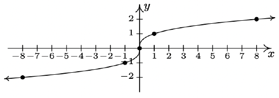
The graph below represents the height \(\ h\) of a Sasquatch (in feet) as a function of its age \(\ N\) in years. Use it to answer the questions in Exercises 86 - 90.

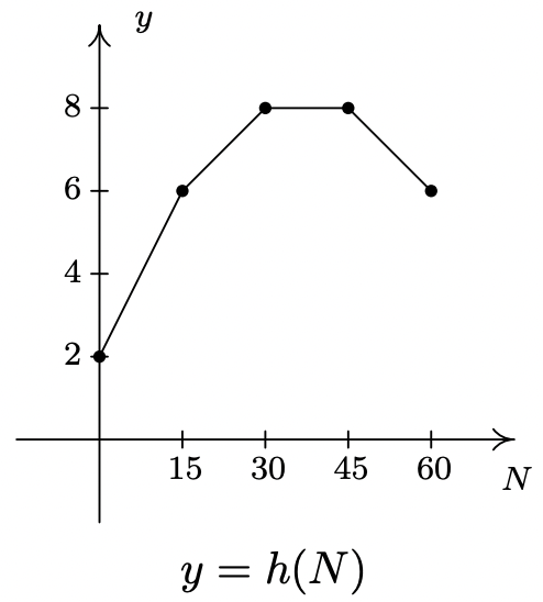
86. Find and interpret \(\ h(0)\).
87. How tall is the Sasquatch when she is 15 years old?
88. Solve \(\ h(N) = 6\) and interpret.
89. List the interval over which \(\ h\) is constant and interpret your answer.
90. List the interval over which \(\ h\) is decreasing and interpret your answer.

For Exercises 91 - 93, let \(\ f(x)=\lfloor x\rfloor\) be the greatest integer function as defined in Exercise 75 in Section 1.4.

91. Graph \(\ y = f(x)\). Be careful to correctly describe the behavior of the graph near the integers.
92. Is \(\ f\) even, odd, or neither? Explain.
93. Discuss with your classmates which points on the graph are local minimums, local maximums or both. Is \(\ f\) ever increasing? Decreasing? Constant?

In Exercises 94 - 95, use graphing technology to show that the given function does not have any extrema, neither local nor absolute.

94. \(\ f(x)=x^{3}+x-12\)
95. \(\ f(x)=-5 x+2\)
96. In Exercise 71 in Section 1.4, we saw that the population of Sasquatch in Portage County could be modeled by the function \(\ P(t)=\frac{150 t}{t+15}\), where \(\ t = 0\) represents the year 1803. Use graphing technology to analyze the general function behavior of \(\ P\). Will there ever be a time when 200 Sasquatch roam Portage County?
97. Suppose \(\ f\) and \(\ g\) are both even functions. What can be said about the functions \(\ f + g\), \(\ f − g\), \(\ fg\) and \(\ \frac{f}{g}\)? What if \(\ f\) and g are both odd? What if f is even but g is odd?
98. One of the most important aspects of the Cartesian Coordinate Plane is its ability to put Algebra into geometric terms and Geometry into algebraic terms. We’ve spent most of this chapter looking at this very phenomenon and now you should spend some time with your classmates reviewing what we’ve done. What major results do we have that tie Algebra and Geometry together? What concepts from Geometry have we not yet described algebraically? What topics from Intermediate Algebra have we not yet discussed geometrically?

It’s now time to “thoroughly vet the pathologies induced” by the precise definitions of local maximum and local minimum. We’ll do this by providing you and your classmates a series of Exercises to discuss. You will need to refer back to the definitions of Increasing, Decreasing and Constant and Maximum and Minimum during the discussion.

99. Consider the graph of the function \(\ f\) given below.

    

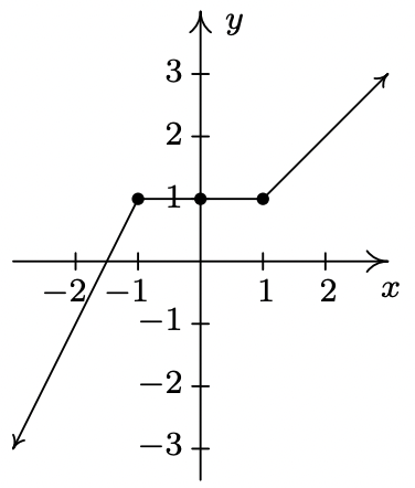
    1. Show that \(\ f\) has a local maximum but not a local minimum at the point (−1, 1).
    2. Show that \(\ f\) has a local minimum but not a local maximum at the point (1, 1).
    3. Show that \(\ f\) has a local maximum AND a local minimum at the point (0, 1).
    4. Show that \(\ f\) is constant on the interval [−1, 1] and thus has both a local maximum AND a local minimum at every point \(\ (x, f(x))\) where \(\ −1 < x < 1\).
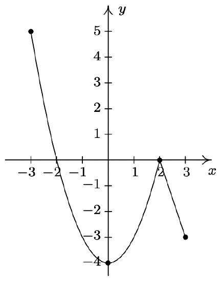
100. Using Example 1.6.4 as a guide, show that the function g whose graph is given below does not have a local maximum at (−3, 5) nor does it have a local minimum at (3, −3). Find its extrema, both local and absolute. What’s unique about the point (0, −4) on this graph? Also find the intervals on which \(\ g\) is increasing and those on which \(\ g\) is decreasing.

     

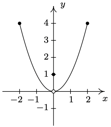
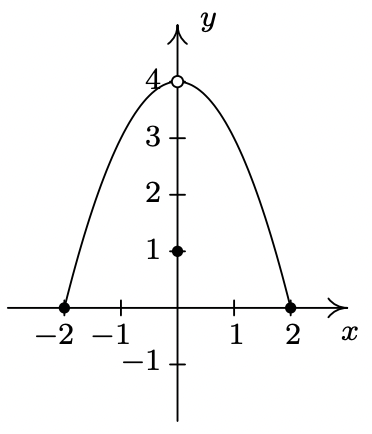
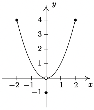
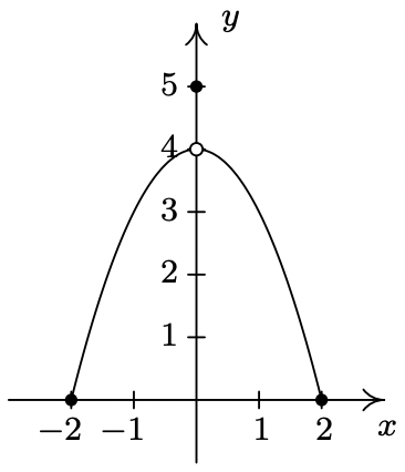
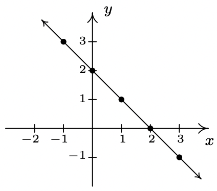
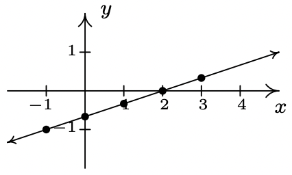
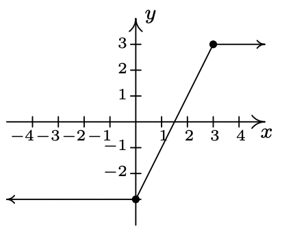
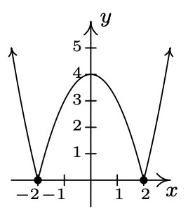
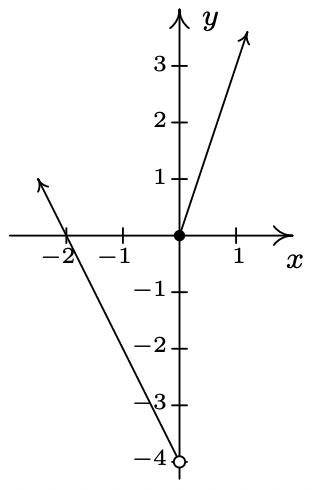
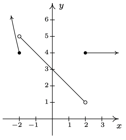
101. We said earlier in the section that it is not good enough to say local extrema exist where a function changes from increasing to decreasing or vice versa. As a previous exercise showed, we could have local extrema when a function is constant so now we need to examine some functions whose graphs do indeed change direction. Consider the functions graphed below. Notice that all four of them change direction at an open circle on the graph. Examine each for local extrema. What is the effect of placing the “dot” on the y-axis above or below the open circle? What could you say if no function value were assigned to \(\ x = 0\)?
     1. Function I

        

     2. Function II

        

     3. Function III

        

     4. Function IV

        

Answers

1. \(\ f(x) = 2 − x\)

   Domain: \\(\ (-\infty, \infty)\)

   x-intercept: (2, 0)

   y-intercept: (0, 2)

   No symmetry

   

2. \(\ f(x)=\frac{x-2}{3}\)

   Domain: \\(\ (-\infty, \infty)\)

   x-intercept: (2, 0)

   y-intercept: \(\ \left(0,-\frac{2}{3}\right)\)

   No symmetr

   

3. \(\ f(x)=x^{2}+1\)

   Domain: \\(\ (-\infty, \infty)\)

   x-intercept: None

   y-intercept: (0, 1)

   Even

   

4. \(\ f(x)=4-x^{2}\)

   Domain: \\(\ (-\infty, \infty)\)

   x-intercepts: (−2, 0), (2, 0)

   y-intercept: (0, 4)

   Even

   

5. \(\ f(x) = 2\)

   Domain: \\(\ (-\infty, \infty)\)

   x-intercept: None

   y-intercept: (0, 2)

   Even

   

6. \(\ f(x)=x^{3}\)

   Domain: \\(\ (-\infty, \infty)\)

   x-intercept: (0, 0)

   y-intercept: (0, 0)

   Odd

   

7. \(\ f(x) = x(x − 1)(x + 2)\)

   Domain: \\(\ (-\infty, \infty)\)

   x-intercepts: (−2, 0), (0, 0), (1, 0)

   y-intercept: (0, 0)

   No symmetry

   

8. \(\ f(x)=\sqrt{x-2}\)

   Domain: \(\[2, \infty)\)

   x-intercept: (2, 0)

   y-intercept: None

   No symmetry

   

9. \(\ f(x)=\sqrt{x-2}\)

   Domain: \(\[2, \infty)\)

   x-intercept: (5, 0)

   y-intercept: \(\ (0, \sqrt{5})\)

   No symmetry

   

10. \(\ f(x)=3-2 \sqrt{x+2}\)

    Domain: \(\ [-2, \infty)\)

    x-intercept: \(\ \left(\frac{1}{4}, 0\right)\)

    y-intercept: \(\ (0,3-2 \sqrt{2})\)

    No symmetry

    

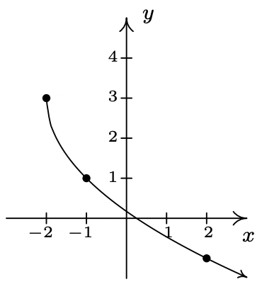
11. \(\ f(x)=\sqrt[3]{x}\)

    Domain: \\(\ (-\infty, \infty)\)

    x-intercept: (0, 0)

    y-intercept: (0, 0)

    Odd

    

12. \(\ f(x)=\frac{1}{x^{2}+1}\)

    Domain: \\(\ (-\infty, \infty)\)

    x-intercept: None

    y-intercept: (0, 1)

    Even

    

13. 
14. 
15. 
16. 
17. 
18. 
19. 
20. 
21. odd
22. neither
23. even
24. even
25. even
26. neither
27. odd
28. odd
29. even
30. neither
31. neither
32. even
33. even and odd
34. odd
35. even
36. even
37. neither
38. odd
39. odd
40. even
41. even
42. [−5, 3]
43. [−5, 4]
44. \(\ f(−2) = 2\)
45. x = −3
46. (−4, 0), (−1, 0), (1, 0)
47. (0, −1)
48. −4, −1, 1
49. \(\ [-4,-1] \cup[1,3]\)
50. 4
51. neither
52. [−5, −3], [0, 2]
53. [−3, 0], [2, 3]
54. \(\ f(−3) = 4, f(2) = 3\)
55. \(\ f(0) = −1\)
56. \(\ f(−3) = 4\)
57. \(\ f(−5) = −5\)
58. [−4, 4]
59. [−5, 5)
60. \(\ f(2) = 3\)
61. x = −2
62. (−4, 0), (0, 0), (4, 0)
63. (0, 0)
64. −4, 0, 4
65. \(\ [-4,0] \cup\{4\}\)
66. 3
67. neither
68. [−2, 2)
69. [−4, −2], (2, 4]
70. none
71. \(\ f(−2) = −5, f(2) = 3\)
72. none
73. \(\ f(−2) = −5\)
74. No absolute maximum

    Absolute minimum \(\ f(4.55) ≈ −175.46\)

    Local minimum at (−2.84, −91.32)

    Local maximum at (0.54, 55.73)

    Local minimum at (4.55, −175.46)

    Increasing on [−2.84, 0.54], [4.55, ∞)

    Decreasing on (−∞, −2.84], [0.54, 4.55]

75. No absolute maximum

    No absolute minimum

    Local maximum at (0, 0)

    Local minimum at (1.60, −3.28)

    Increasing on (−∞, 0], [1.60, ∞)

    Decreasing on [0, 1.60]

76. Absolute maximum \(\ f(0) = 3\)

    Absolute minimum f(±3) = 0

    Local maximum at (0, 3)

    No local minimum

    Increasing on [−3, 0]

    Decreasing on [0, 3]

77. Absolute maximum f(2.12) ≈ 4.50

    Absolute minimum f(−2.12) ≈ −4.50

    Local maximum (2.12, 4.50)

    Local minimum (−2.12, −4.50)

    Increasing on [−2.12, 2.12]

    Decreasing on [−3, −2.12], [2.12, 3]

78. \(\ (f + g)(0) = 4\)
79. \(\ (f + g)(1) = 5\)
80. \(\ (f − g)(1) = −1\)
81. \(\ (g − f)(2) = 0\)
82. \(\ (fg)(2) = 9\)
83. \(\ (fg)(1) = 6\)
84. \(\ \left(\frac{f}{g}\right)(4)=0\)
85. \(\ \left(\frac{g}{f}\right)(2)=1\)
86. \(\ h(0) = 2\), so the Sasquatch is 2 feet tall at birth.
87. \(\ h(15) = 6\), so the Saquatch is 6 feet tall when she is 15 years old.
88. \(\ h(N) = 6\) when \(\ N = 15\) and \(\ N = 60\). This means the Sasquatch is 6 feet tall when she is 15 and 60 years old.
89. \(\ h\) is constant on [30, 45]. This means the Sasquatch’s height is constant (at 8 feet) for these years.
90. \(\ h\) is decreasing on [45, 60]. This means the Sasquatch is getting shorter from the age of 45 to the age of 60. (Sasquatchteoporosis, perhaps?)
91. 
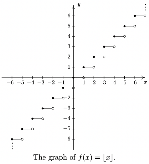
92. Note that \(\ f(1.1) = 1\), but \(\ f(−1.1) = −2\), so f is neither even nor odd.