
1.7: Transformations
- Page ID
- 120120

\( \newcommand{\vecs}[1]{\overset { \scriptstyle \rightharpoonup} {\mathbf{#1}} } \)
\( \newcommand{\vecd}[1]{\overset{-\!-\!\rightharpoonup}{\vphantom{a}\smash {#1}}} \)
\( \newcommand{\dsum}{\displaystyle\sum\limits} \)
\( \newcommand{\dint}{\displaystyle\int\limits} \)
\( \newcommand{\dlim}{\displaystyle\lim\limits} \)
\( \newcommand{\id}{\mathrm{id}}\) \( \newcommand{\Span}{\mathrm{span}}\)
( \newcommand{\kernel}{\mathrm{null}\,}\) \( \newcommand{\range}{\mathrm{range}\,}\)
\( \newcommand{\RealPart}{\mathrm{Re}}\) \( \newcommand{\ImaginaryPart}{\mathrm{Im}}\)
\( \newcommand{\Argument}{\mathrm{Arg}}\) \( \newcommand{\norm}[1]{\| #1 \|}\)
\( \newcommand{\inner}[2]{\langle #1, #2 \rangle}\)
\( \newcommand{\Span}{\mathrm{span}}\)
\( \newcommand{\id}{\mathrm{id}}\)
\( \newcommand{\Span}{\mathrm{span}}\)
\( \newcommand{\kernel}{\mathrm{null}\,}\)
\( \newcommand{\range}{\mathrm{range}\,}\)
\( \newcommand{\RealPart}{\mathrm{Re}}\)
\( \newcommand{\ImaginaryPart}{\mathrm{Im}}\)
\( \newcommand{\Argument}{\mathrm{Arg}}\)
\( \newcommand{\norm}[1]{\| #1 \|}\)
\( \newcommand{\inner}[2]{\langle #1, #2 \rangle}\)
\( \newcommand{\Span}{\mathrm{span}}\) \( \newcommand{\AA}{\unicode[.8,0]{x212B}}\)
\( \newcommand{\vectorA}[1]{\vec{#1}} % arrow\)
\( \newcommand{\vectorAt}[1]{\vec{\text{#1}}} % arrow\)
\( \newcommand{\vectorB}[1]{\overset { \scriptstyle \rightharpoonup} {\mathbf{#1}} } \)
\( \newcommand{\vectorC}[1]{\textbf{#1}} \)
\( \newcommand{\vectorD}[1]{\overrightarrow{#1}} \)
\( \newcommand{\vectorDt}[1]{\overrightarrow{\text{#1}}} \)
\( \newcommand{\vectE}[1]{\overset{-\!-\!\rightharpoonup}{\vphantom{a}\smash{\mathbf {#1}}}} \)
\( \newcommand{\vecs}[1]{\overset { \scriptstyle \rightharpoonup} {\mathbf{#1}} } \)
\(\newcommand{\longvect}{\overrightarrow}\)
\( \newcommand{\vecd}[1]{\overset{-\!-\!\rightharpoonup}{\vphantom{a}\smash {#1}}} \)
\(\newcommand{\avec}{\mathbf a}\) \(\newcommand{\bvec}{\mathbf b}\) \(\newcommand{\cvec}{\mathbf c}\) \(\newcommand{\dvec}{\mathbf d}\) \(\newcommand{\dtil}{\widetilde{\mathbf d}}\) \(\newcommand{\evec}{\mathbf e}\) \(\newcommand{\fvec}{\mathbf f}\) \(\newcommand{\nvec}{\mathbf n}\) \(\newcommand{\pvec}{\mathbf p}\) \(\newcommand{\qvec}{\mathbf q}\) \(\newcommand{\svec}{\mathbf s}\) \(\newcommand{\tvec}{\mathbf t}\) \(\newcommand{\uvec}{\mathbf u}\) \(\newcommand{\vvec}{\mathbf v}\) \(\newcommand{\wvec}{\mathbf w}\) \(\newcommand{\xvec}{\mathbf x}\) \(\newcommand{\yvec}{\mathbf y}\) \(\newcommand{\zvec}{\mathbf z}\) \(\newcommand{\rvec}{\mathbf r}\) \(\newcommand{\mvec}{\mathbf m}\) \(\newcommand{\zerovec}{\mathbf 0}\) \(\newcommand{\onevec}{\mathbf 1}\) \(\newcommand{\real}{\mathbb R}\) \(\newcommand{\twovec}[2]{\left[\begin{array}{r}#1 \\ #2 \end{array}\right]}\) \(\newcommand{\ctwovec}[2]{\left[\begin{array}{c}#1 \\ #2 \end{array}\right]}\) \(\newcommand{\threevec}[3]{\left[\begin{array}{r}#1 \\ #2 \\ #3 \end{array}\right]}\) \(\newcommand{\cthreevec}[3]{\left[\begin{array}{c}#1 \\ #2 \\ #3 \end{array}\right]}\) \(\newcommand{\fourvec}[4]{\left[\begin{array}{r}#1 \\ #2 \\ #3 \\ #4 \end{array}\right]}\) \(\newcommand{\cfourvec}[4]{\left[\begin{array}{c}#1 \\ #2 \\ #3 \\ #4 \end{array}\right]}\) \(\newcommand{\fivevec}[5]{\left[\begin{array}{r}#1 \\ #2 \\ #3 \\ #4 \\ #5 \\ \end{array}\right]}\) \(\newcommand{\cfivevec}[5]{\left[\begin{array}{c}#1 \\ #2 \\ #3 \\ #4 \\ #5 \\ \end{array}\right]}\) \(\newcommand{\mattwo}[4]{\left[\begin{array}{rr}#1 \amp #2 \\ #3 \amp #4 \\ \end{array}\right]}\) \(\newcommand{\laspan}[1]{\text{Span}\{#1\}}\) \(\newcommand{\bcal}{\cal B}\) \(\newcommand{\ccal}{\cal C}\) \(\newcommand{\scal}{\cal S}\) \(\newcommand{\wcal}{\cal W}\) \(\newcommand{\ecal}{\cal E}\) \(\newcommand{\coords}[2]{\left\{#1\right\}_{#2}}\) \(\newcommand{\gray}[1]{\color{gray}{#1}}\) \(\newcommand{\lgray}[1]{\color{lightgray}{#1}}\) \(\newcommand{\rank}{\operatorname{rank}}\) \(\newcommand{\row}{\text{Row}}\) \(\newcommand{\col}{\text{Col}}\) \(\renewcommand{\row}{\text{Row}}\) \(\newcommand{\nul}{\text{Nul}}\) \(\newcommand{\var}{\text{Var}}\) \(\newcommand{\corr}{\text{corr}}\) \(\newcommand{\len}[1]{\left|#1\right|}\) \(\newcommand{\bbar}{\overline{\bvec}}\) \(\newcommand{\bhat}{\widehat{\bvec}}\) \(\newcommand{\bperp}{\bvec^\perp}\) \(\newcommand{\xhat}{\widehat{\xvec}}\) \(\newcommand{\vhat}{\widehat{\vvec}}\) \(\newcommand{\uhat}{\widehat{\uvec}}\) \(\newcommand{\what}{\widehat{\wvec}}\) \(\newcommand{\Sighat}{\widehat{\Sigma}}\) \(\newcommand{\lt}{<}\) \(\newcommand{\gt}{>}\) \(\newcommand{\amp}{&}\) \(\definecolor{fillinmathshade}{gray}{0.9}\)The following topics related to the material in this section are assumed prerequisites for this course. They are only covered if you are enrolled in a class with corequisite support:
- Graphing the eight base functions: \( y = x \), \( y = x^2 \), \( y = x^3 \), \( y = \sqrt{x} \), \( y = \sqrt[3]{x} \), \( y = |x| \), \( y = \frac{1}{x} \), and \( y = \frac{1}{x^2} \)
- Graphing functions involving rigid transformations (including vertical reflections)
- Graphical functions involving non-rigid transformation that are vertical scalings
- Graph functions involving multiple algebraic transformations, including shifts, reflections, and scalings.
General Form of a Transformed Function
In this section, we review how to graph the transformation of a function \( f \). Suppose\[ h(x) = A f(B x + C) + D, \label{trans1} \]where \( A \), \( B \), \( C \), and \( D \) are real numbers, \( A \neq 0 \) and \( B \neq 0 \), and where \( f(x) \) is a function whose graph we are familiar with or have been given. In this case, the graph of \( f \) is called the base graph for \( h \) as it is the graph we manipulate to eventually arrive at the graph of \( h \). We will refer to the form presented in Equation \ref{trans1} as the general form of the transformed function \( f \). Throughout this section, we will explore the effects that the constants \( A \), \( B \), \( C \), and \( D \) have on the graphing process. Since you have already learned this topic in your previous Algebra courses, we will take a "higher-level" approach here.
While going through this section's theory, we will often refer to the following two graphs.
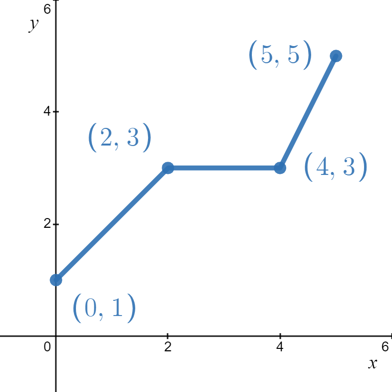
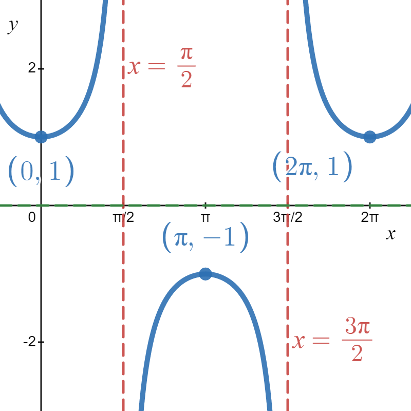
Figure \( \PageIndex{1A} \) (left): the base graph \( f(x) \)
Figure \( \PageIndex{1B} \) (right): the base graph \( g(x) = \sec{(x)} \)
Recall that the Fundamental Graphing Principle for Functions states for a point \((x_1, y_1)\) to be on the graph of the function, \(f(x_1) = y_1\).1 In particular, from Figure \( \PageIndex{1A} \) we know \(f(0) = 1\), \(f(2)=3\), \(f(4)=3\) and \(f(5)=5\). From Figure \( \PageIndex{1B} \), we have three anchor points,2 \( g(0) = 1 \), \( g(\pi) = -1 \), and \( g(2 \pi) = 1 \). The graph of \( g(x) = \sec{(x)} \) also shows two of the secant's (infinitely many) vertical asymptotes, \( x = \frac{\pi}{2} \) and \( x = \frac{3 \pi}{2} \), dashed in red along with the "midline" of \( y = 0 \) dashed in green.3 With that in mind, we begin our "high-level" review of transformations.
The Order of Transformations
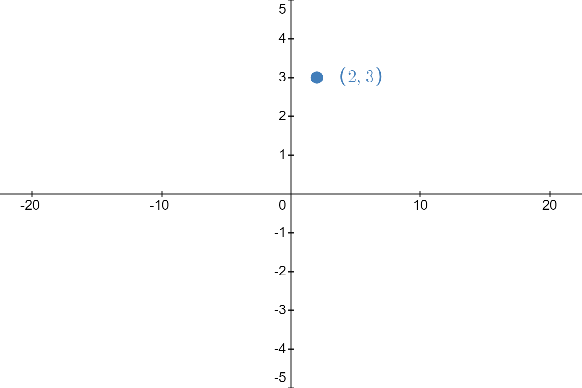
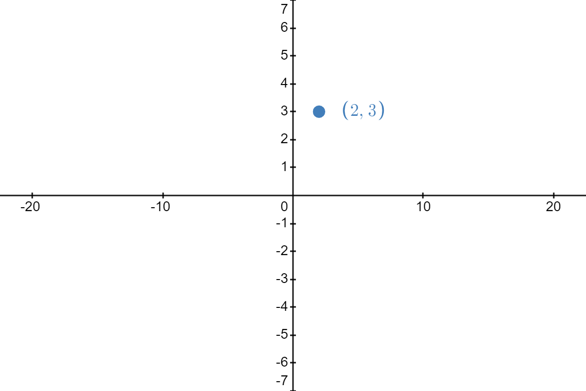
To be honest, there is not one agreed-upon "order" with which to perform transformations; however, every approach presented by mathematicians across the globe takes into consideration the ramifications of the order they have selected. For example, suppose you have the point \( (2,3) \) from the graph of \( f(x) \) in Figure \( \PageIndex{1A} \) and you are asked to perform the following transformations:
- reflect the point across the \( x \)-axis
- compress the point vertically by a factor of \( \frac{1}{3} \)
- reflect the point across the \( y \)-axis
- stretch the point horizontally by a factor of \( 4 \)
- shift the point up \( 3 \) units
- shift the point left \( 5 \) units
Performing these operations in the order listed gives the following result:
 |
\( \underrightarrow{\text{reflect about }x\text{-axis}} \) | 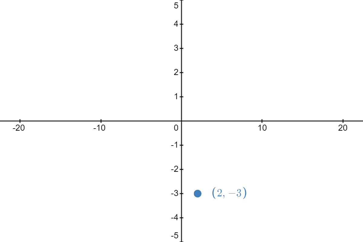 |
| \( \underrightarrow{\text{compress vertically by factor of }\frac{1}{3}} \) | 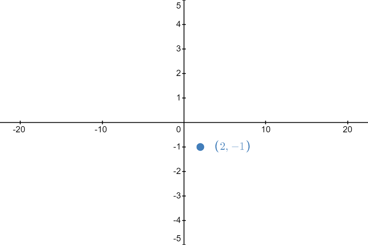 |
|
| \( \underrightarrow{\text{reflect about }y\text{-axis}} \) | 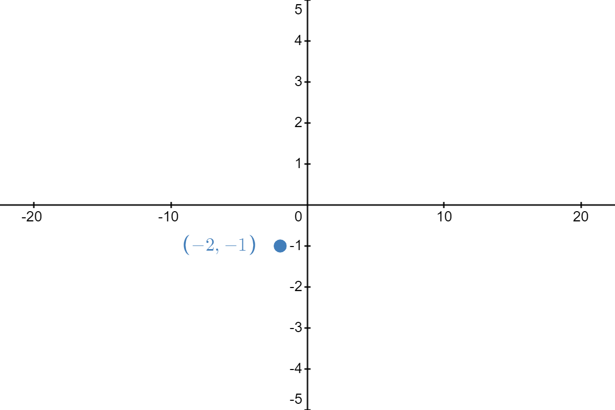 |
|
| \( \underrightarrow{\text{stretch horizontally by factor of }4} \) | 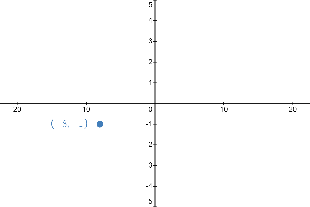 |
|
| \( \underrightarrow{\text{shift up }3\text{ units}} \) | 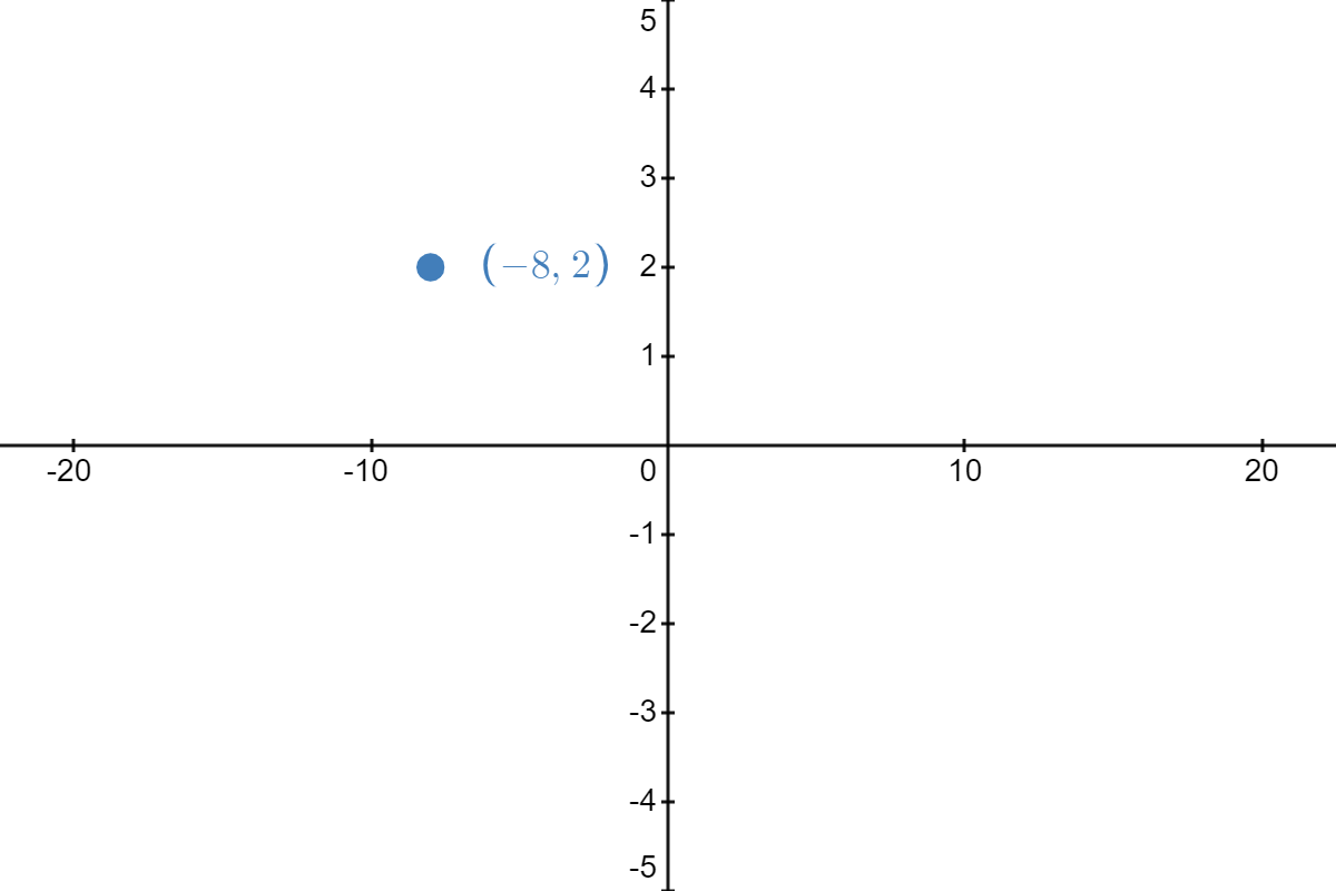 |
|
| \( \underrightarrow{\text{shift left }5\text{ units}} \) | 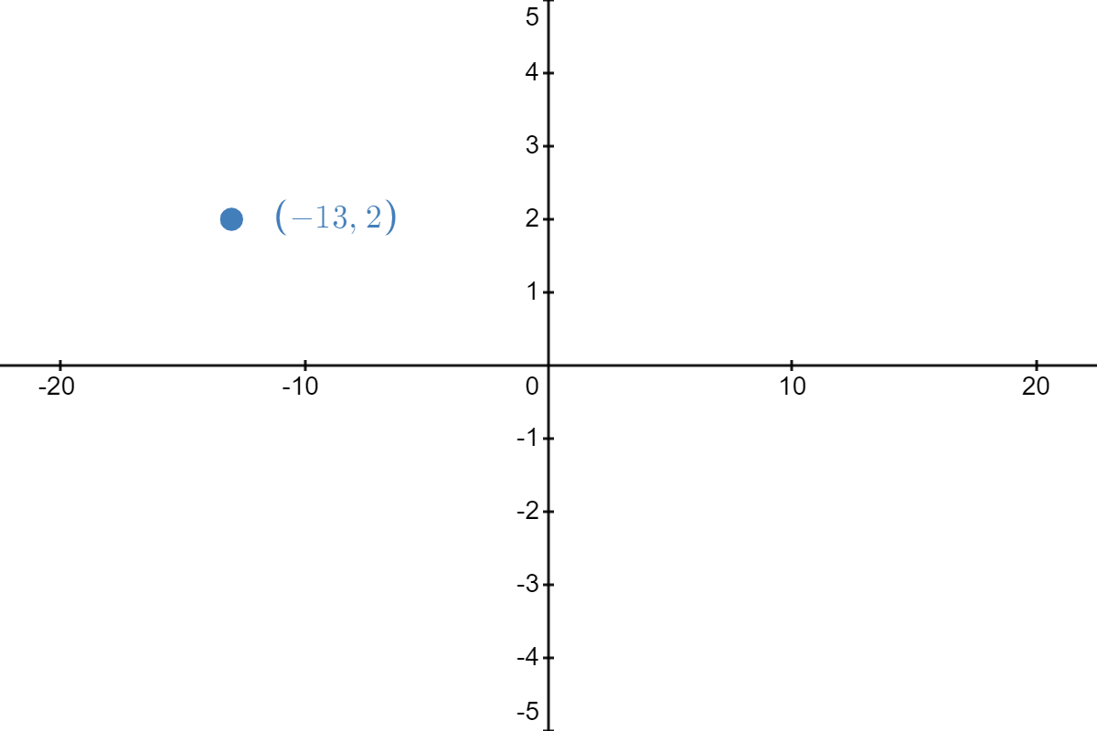 |
Thus, the result of all of these transformations, in the order listed, is to take the point \( (2,3) \) on our graph of \( f \) and manipulate it to become \( (-13,2) \) on the graph of \( h \).
Before continuing, let's make a critical clarification. When I say "compress vertically by a factor of \( \frac{1}{3} \)," I mean "squish" the \( y \)-values toward the \( x \)-axis by multiplying them by \( \frac{1}{3} \). Likewise, when I say "stretch horizontally by a factor of \( 4 \)," I mean "pull" the \( x \)-values away from the \( y \)-axis by multiplying them by \( 4 \).
Had we done things in a different order, would we have arrived at the same result? Well, there's no better teacher than experience, so let's see by experimenting.
 |
\( \underrightarrow{\text{shift up }3\text{ units}} \) | 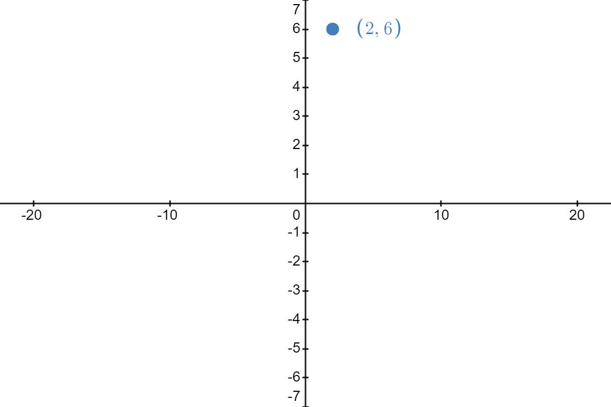 |
| \( \underrightarrow{\text{shift left }5\text{ units}} \) | 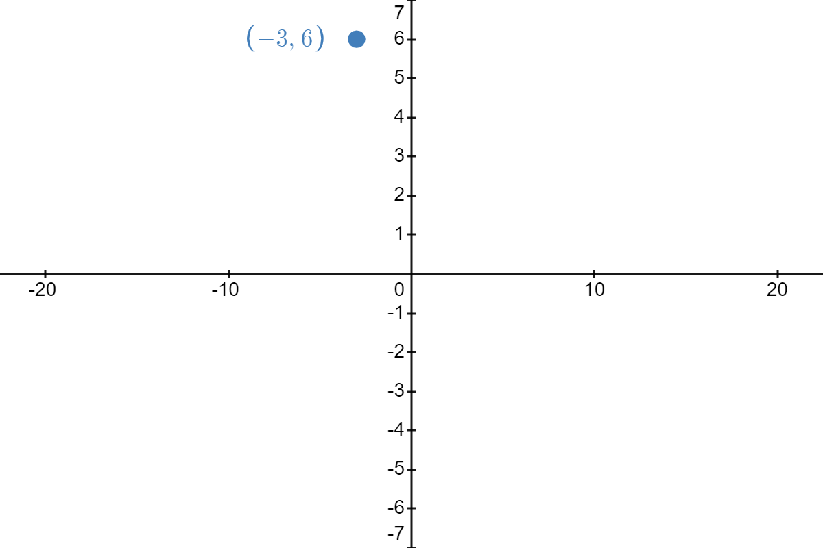 |
|
| \( \underrightarrow{\text{reflect about }x\text{-axis}} \) | 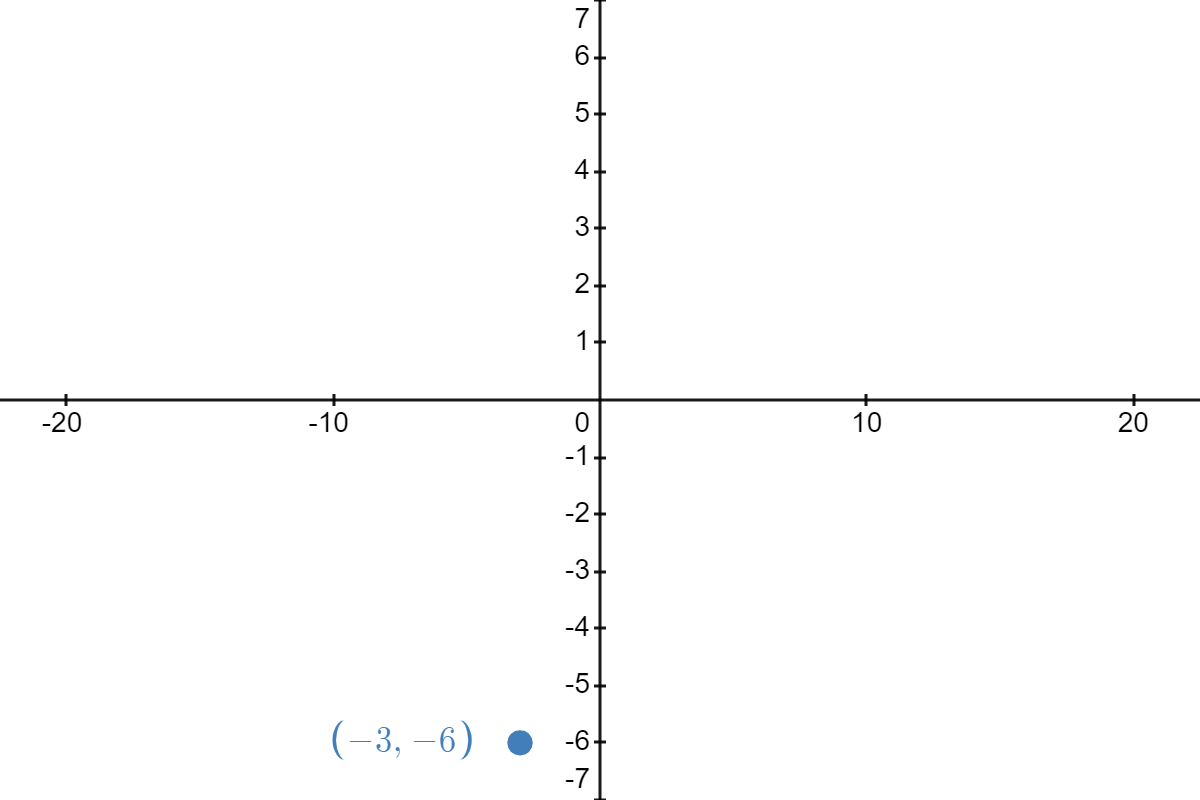 |
|
| \( \underrightarrow{\text{compress vertically by factor of }\frac{1}{3}} \) | 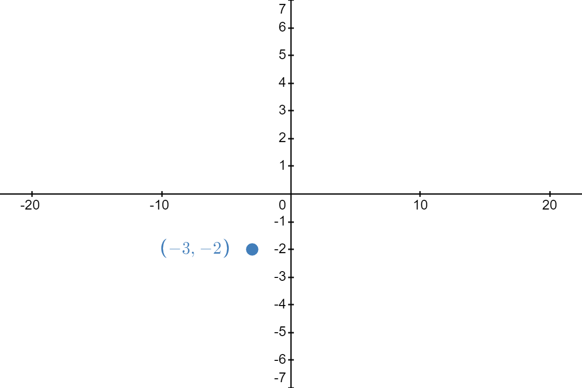 |
|
| \( \underrightarrow{\text{reflect about }y\text{-axis}} \) | 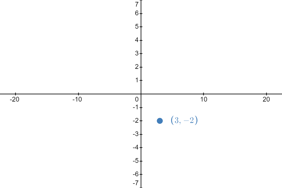 |
|
| \( \underrightarrow{\text{stretch horizontally by factor of }4} \) | 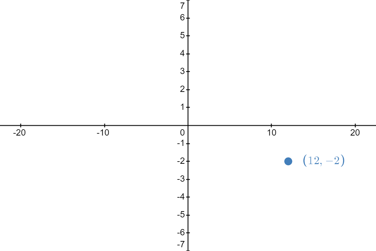 |
As we can see, switching the order changes the resulting point to \( (12, -2) \), which is definitely not \( (-13,2) \).
So, how do we guarantee that we are always performing the transformations in the correct order?
There is something akin to the Order of Operations for transformations. Given the transformation of \( f \) in Equation \ref{trans1}, we focus on \( x \) and perform the Order of Operations on \( x \).4\[ h(x) = A f\left(B \boxed{x} + C\right) + D \nonumber \]According to the Order of Operations, if an exponent or some other function were acting on \( x \), we would apply it, but the only things happening to \( x \) inside those parentheses is multiplication by \( B \) and an addition by \( C \). Multiplication beats addition, so let's perform the multiplication first.\[ h(x) = A f\left(\boxed{Bx} + C\right) + D \nonumber \]Continuing on with the Order of Operations, we add the \( C \).\[ h(x) = A f\left(\boxed{Bx + C}\right) + D \nonumber \]Moving outside of the function, we see \( f \) is being multiplied by \( A \) and added to by \( D \).5 Again, following the Order of Operations, we apply the multiplication first.\[ h(x) = \boxed{A f\left(Bx + C\right)} + D \nonumber \]Finally, there is nothing left but to apply the addition.\[ h(x) = \boxed{A f\left(Bx + C\right) + D} \nonumber \]What we have witnessed is exactly how we will apply our transformations in this text. I call this the "Order of Transformations."
Let \( h(x) \) be a function that can be written as\[ h(x) = A f(Bx + C) + D, \nonumber \]for constants \( A \), \( B \), \( C \), and \( D \), where \( A \neq 0 \) and \( B \neq 0 \). The graph of \( h \) can be obtained from the graph of \( f \) as follows:
- apply the transformation associated with the multiplication of \( x \) by \( B \)
- apply the transformation associated with adding \( C \) to \( Bx \)
- apply the transformation associated with the multiplication of \( f(Bx + C) \) by \( A \)
- apply the transformation associated with adding \( D \) to \( A f(B x + C) \)
There are a few items to point out here. First, we have not stated yet, nor have we proved, what effects each of these transformations has on the graphing process. All we "officially" know at this point is that, according to the Order of Transformations (which is based on the Order of Operations), we should apply the transformation associated with \( B \), then \( C \), then \( A \), and finally \( D \) - in that order.6
Second, in Step 2 of the Order of Transformations, we "apply the transformation associated with adding \( C \) to \(Bx \)" - not to \( x \). As we will see, this is going to necessitate some factoring because working with \( Bx \) is more challenging than working with \( x \). Therefore, in practice, we rewrite Equation \ref{trans1} in the better7 form\[ h(x) = A f\left( B \left( x + \frac{C}{B} \right) \right) + D. \label{trans2} \]We will call this the standard form of the transformed function \( f \).8
Vertical Shifts
Suppose we wanted to graph the function defined by the formula \(h(x) = f(x) + 2\), where \( f \) is the function from Figure \( \PageIndex{1A} \). Let's take a minute to remind ourselves of what \(h\) is doing. We start with an input \(x\) to the function \(f\) and we obtain the output \(f(x)\). The function \(h\) takes the output \(f(x)\) and adds \(2\) to it. In order to graph \(h\), we need to graph the points \((x,h(x))\). How are we to find the values for \(h(x)\) without a formula for \(f(x)\)? The answer is that we don't need a formula for \(f(x)\); we need the values of \(f(x)\). The values of \(f(x)\) are the \(y\) values on the graph of \(y=f(x)\). For example, we can make the following table using the points indicated on the graph of \(f\).\[\begin{array}{|c|c|c|}
\hline x & f(x) & h(x)=f(x)+2 \\
\hline 0 & 1 & 3 \\
\hline 2 & 3 & 5 \\
\hline 4 & 3 & 5 \\
\hline 5 & 5 & 7 \\
\hline \end{array}\nonumber\]In general, if \((x_1,y_1)\) is on the graph of \(y=f(x)\), then \(f(x_1) = y_1\), so \(g(x_1) = f(x_1) +2 = y_1+2\). Hence, \((x_1 ,y_1+2)\) is on the graph of \(h\).
In other words, to obtain the graph of \(h\), we add \(2\) to the \(y\)-coordinate of each point on the graph of \(f\). Geometrically, adding \(2\) to the \(y\)-coordinate of a point moves the point \(2\) units above its previous location. Adding \(2\) to every \(y\)-coordinate on a graph en masse is usually described as "shifting the graph up \(2\) units." Notice that the graph retains the same basic shape as before, it is just \(2\) units above its original location. We see the results in Figure \( \PageIndex{2A} \).
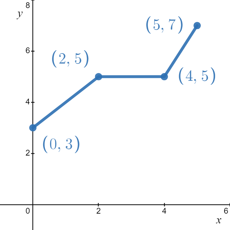
Figure \( \PageIndex{2A} \): \( h(x) = f(x) + 2 \)
You’ll note that the domain of \(f\) and the domain of \(h\) are the same, namely \([0,5]\), but that the range of \(f\) is \([1,5]\) while the range of \(h\) is \([3,7]\). In general, shifting a function vertically like this will leave the domain unchanged, but could very well affect the range.
Suppose we want to graph the function \(j(x) = g(x) - 2\), where \( g \) is the secant function in Figure \( \PageIndex{1B} \). Instead of adding \(2\) to each of the \(y\)-coordinates on the graph of \(g\), we’d subtract \(2\). Geometrically, we move the graph down \(2\) units. The domain of \(j\) is the same as \(g\), but the range of \(j\) is \((-\infty, -3] \cup [-1,\infty)\) (instead of \( (-\infty, -1] \cup [1, \infty) \)). In this case, since our original graph had a "midline," we also move that down \( 2 \) units. We see the results in Figure \( \PageIndex{2B}\).
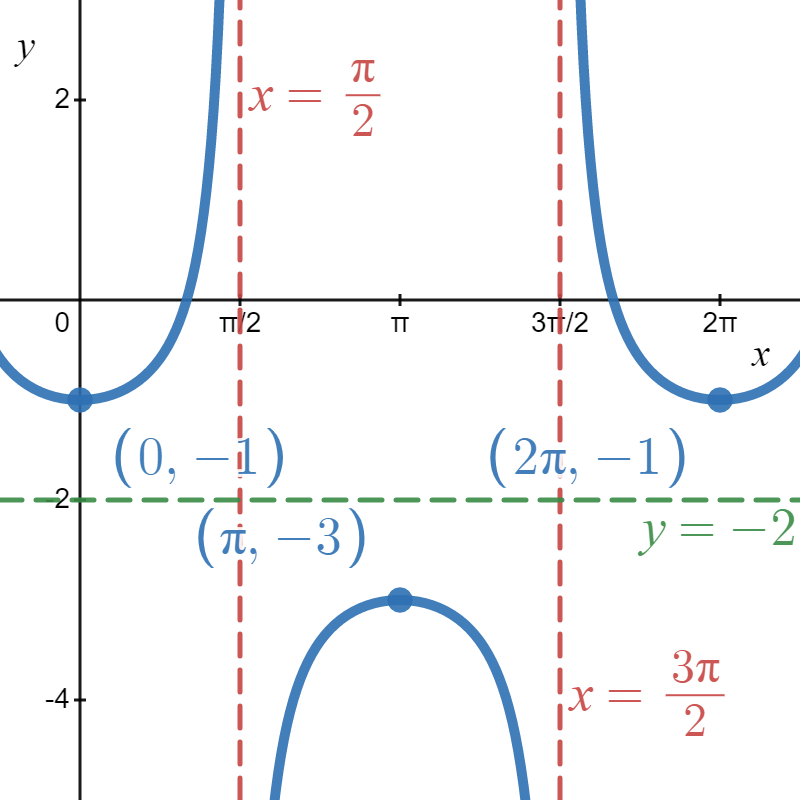
Figure \( \PageIndex{2B} \): \( j(x) = g(x) - 2 = \sec{(x)} - 2 \)
What we have discussed is generalized in the following theorem.
Suppose \(f\) is a function and \(D\) is a positive number.
- The graph of \(y=f(x)+D\) is obtained from shifting the graph of \(y=f(x)\) up \(D\) units by adding \(D\) to the \(y\)-coordinates of the points on the graph of \(f\).
- The graph of \(y=f(x)-D\) is obtained from shifting the graph of \(y=f(x)\) down \(D\) units by subtracting \(D\) from the \(y\)-coordinates of the points on the graph of \(f\).
The key to understanding this theorem and, indeed, all of the theorems in this section comes from an understanding of the Fundamental Graphing Principle for Functions: If \((x_1, y_1)\) is on the graph of \(f\), then \(f(x_1) = y_1\).
Substituting \(x_1\) into the equation \(y=f(x)+D\) gives \(y=f(x_1)+D = y_1 + D\). Hence, \((x_1,y_1 + D)\) is on the graph of \(y=f(x)+D\), and we have the result. In the language of "inputs" and "outputs," this theorem can be paraphrased as "Adding to, or subtracting from, the output of a function causes the graph to shift up or down, respectively."
Recalling the Order of Transformations, the theorem concerning vertical shifts implies that the vertical shift is the last transformation we perform when graphing the transformation\[ h(x) = A f(Bx + C) + D. \nonumber \]
Horizontal Shifts
When working on the "outside" of a function, we are concerned with the changes in the \( y \)-values corresponding to our static \( x \)-values. That is, in the previous discussion, we determined the new \( y \)-values for both \( h(x) \) and \( j(x) \) corresponding to the original, static \( x \)-values on the graphs of \( f(x) \) and \( g(x) \), respectively. As we shall see when working on the "inside" of a function, we are concerned with how we need to change the \( x \)-values to arrive at our static \( y \)-values. You probably have never thought of transformations this way, so we will take our time here.
Keeping with the graph of \(y=f(x)\) in Figure \( \PageIndex{1A} \), suppose we wanted to graph \(h(x) = f(x + 2)\). In other words, we are looking to see what happens when we add \(2\) to the input of the function. We have spent a lot of time in this text showing you that \(\ f(x + 2)\) and \(\ f(x) + 2\) are, in general, wildly different algebraic animals. We will see momentarily that their geometry is also dramatically different.
Let’s try to generate a table of values of \(h\) based on those we know for \(f\). We quickly find that we run into some difficulties.\[\begin{array}{|c|c|c|}
\hline x & f(x) & h(x)=f(x+2) \\
\hline 0 & 1 & f(0+2) = f(2) = 3 \\
\hline 2 & 3 & f(2+2) = f(4) = 3 \\
\hline 4 & 3 & f(4+2) = f(6) = ? \\
\hline 5 & 5 & f(5+2) = f(7) = ? \\
\hline \end{array} \nonumber \]When we substitute \(x=4\) into the formula \(h(x)=f(x+2)\), we are asked to find \(f(4+2)=f(6)\) which doesn’t exist because the domain of \(f\) is only \([0,5]\). The same thing happens when we attempt to find \(h(5)\). What we need here is a new strategy.
We know, for instance, \(f(0) = 1\). To determine the corresponding point on the graph of \(h\), we need to figure out what value of \(x\) we must substitute into \(h(x) = f(x+2)\) so that the quantity \(x+2\), works out to be \(0\). Solving \(x+2=0\) gives \(x=-2\), and \[h(-2) = f((-2)+2) = f(0) = 1\nonumber\]so \((-2,1)\) is on the graph of \(h\). To use the fact \(f(2) = 3\), we set \(x+2 = 2\) to get \(x=0\). Substituting gives \[h(0) = f(0+2) = f(2) = 3.\nonumber\]Continuing in this fashion, we get\[\begin{array}{|c|c|c|}
\hline x & x+2 & h(x)=f(x+2) \\
\hline -2 & 0 & h(-2)=f(0) = 1 \\
\hline 0 & 2 & h(0)=f(2) = 3 \\
\hline 2 & 4 & h(2)=f(4) = 3 \\
\hline 3 & 5 & h(3)=f(5) = 5 \\
\hline \end{array} \nonumber \]In summary, the points \((0,1)\), \((2,3)\), \((4,3)\) and \((5,5)\) on the graph of \(y=f(x)\) give rise to the points \((-2,1)\), \((0,3)\), \((2,3)\) and \((3,5)\) on the graph of \(y=h(x)\), respectively.
Again, leaning on the Fundamental Graphing Principle for Functions, if \((x_1, y_1)\) is on the graph of \(y=f(x)\), then \(f(x_1) = y_1\). Solving \(x + 2 = x_1\) gives \(x = x_1 - 2\) so that \(h(x_1 - 2) = f((x_1-2)+2) = f(x_1) = y_1\). As such, \((x_1-2,y_1)\) is on the graph of \(y=h(x)\). The point \((x_1-2,y_1)\) is exactly \(2\) units to the left of the point \((x_1,y_1)\) so the graph of \(y=h(x)\) is obtained by shifting the graph \(y=f(x)\) to the left \(2\) units, as shown in Figure \( \PageIndex{3A} \).
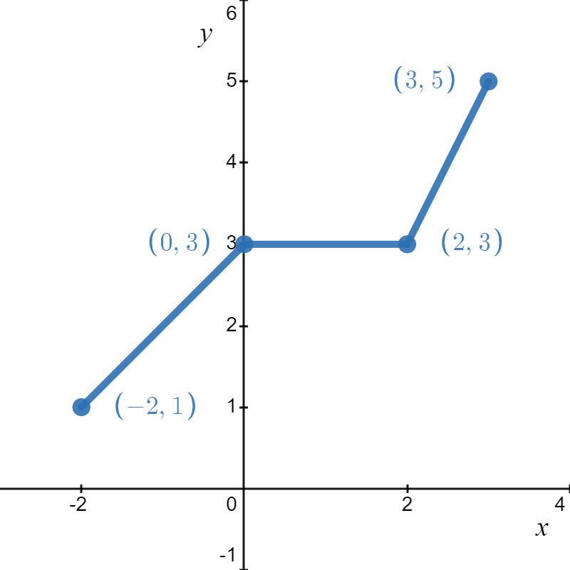
Figure \( \PageIndex{3A} \): \( h(x) = f(x + 2) \)
Note that while the ranges of \(f\) and \(h\) are the same, the domain of \(h\) is \([-2,3]\) whereas the domain of \(f\) is \([0,5]\). In general, when we shift the graph horizontally, the range will remain the same, but the domain could change.
If we graph \(j(x) = g\left(x-\frac{\pi}{4}\right)\), we find ourselves adding \(\frac{\pi}{4}\) to all of the \(x\) values of the points on the graph of \(y=g(x)\) to effect a shift to the right \(\frac{\pi}{4}\) units. In this process, we move the vertical asymptotes to the right \( \frac{\pi}{4} \) units as well, as shown in Figure \( \PageIndex{3B} \).
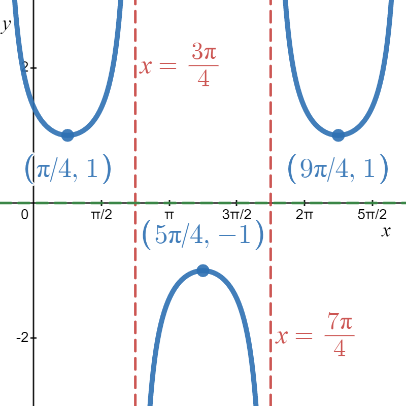
Figure \( \PageIndex{3B} \): \( j(x) = g\left( x - \frac{\pi}{4} \right) = \sec{\left( x - \frac{\pi}{4} \right)} \)
Generalizing these notions produces the following result.
Suppose \(f\) is a function and \(C\) is a positive number.
- The graph of \(y=f(x+C)\) is obtained from shifting the graph of \(y=f(x)\) left \(C\) units by subtracting \(C\) from the \(x\)-coordinates of the points on the graph of \(f\).
- The graph of \(y=f(x-C)\) is obtained from shifting the graph of \(y=f(x)\) right \(C\) units by adding \(C\) to the \(x\)-coordinates of the points on the graph of \(f\).
In other words, adding to or subtracting from the input to a function amounts to shifting the graph left or right, respectively.
This theorem states the graph of \(y=f(x \pm C)\) is obtained from shifting the graph of \(y=f(x)\) left or right \(C\) units; however, it says nothing about the graph of \( y = f(Bx \pm C) \). Suppose the coefficient of \( x \) is something other than \( 1 \). In that case, you must factor the argument to get the function in the form\[ h(x) = A f \left( B \left( x + \frac{C}{B} \right) \right) + D \nonumber \]so that you can see the true shift on \( x \) (not on \( Bx \)). Examples \( \PageIndex{2} \) and \( \PageIndex{3} \) showcase that the true horizontal shift in these cases is \( \pm \frac{C}{B} \).
The previous two theorems concerning vertical and horizontal shifts present a theme that will run throughout the section: changes to the outputs from a function affect the \(y\)-coordinates of the graph, resulting in some vertical change; changes to the inputs to a function affect the \(x\)-coordinates of the graph, resulting in some kind of horizontal change.
Returning to the Order of Transformations, we now know that to graph\[ h(x) = f(x + C) + D, \nonumber \]we apply the horizontal shift, \( C \), and then the vertical shift, \( D \).9
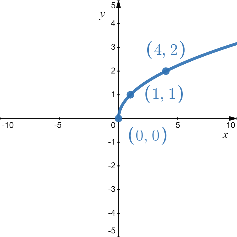
- Graph \(f(x) = \sqrt{x}\). Plot at least three points. State the domain and range of \( f \).
- Use your graph in 1 to graph \(g(x) = \sqrt{x}-1\). State the domain and range of \( g \).
- Use your graph in 1 to graph \(j(x) = \sqrt{x-1}\). State the domain and range of \( j \).
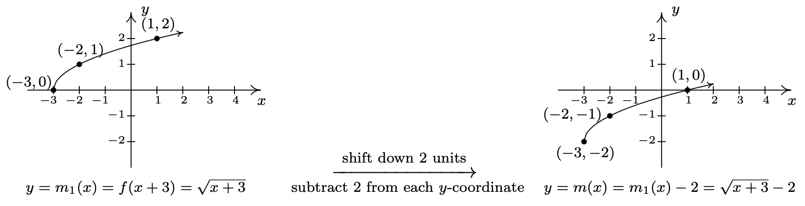
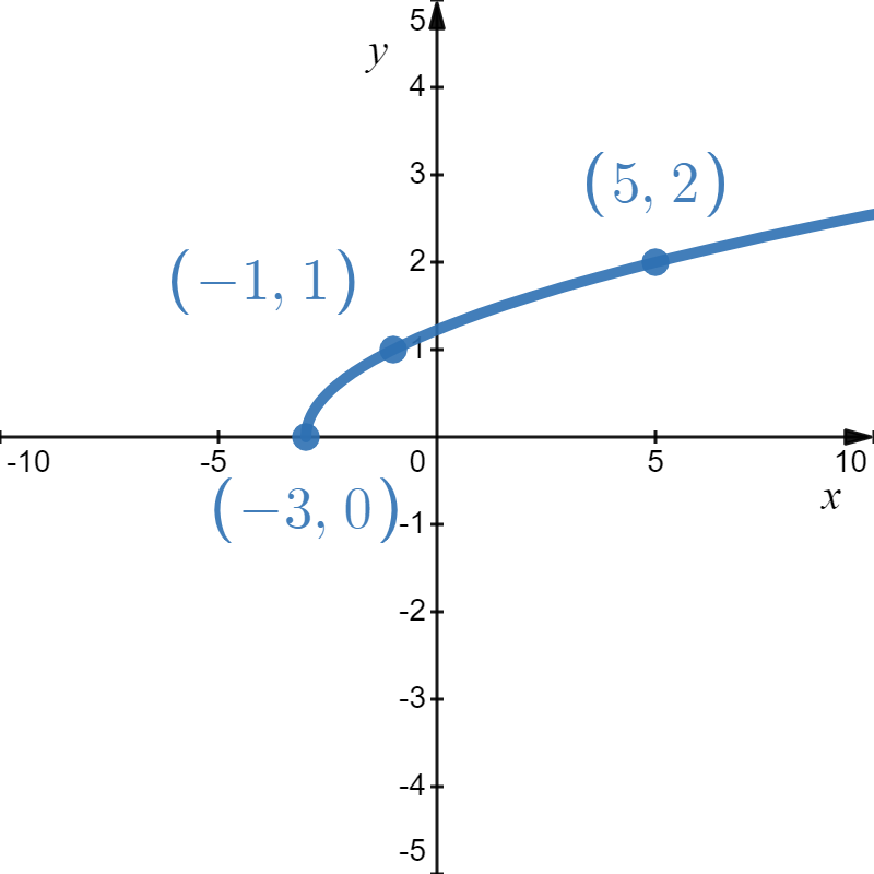
- Use your graph in 1 to graph \(m(x) = \sqrt{x+3} - 2\). State the domain and range of \( m \).
- Solutions
-
- Owing to the square root, the domain of \(f\) is \(x \geq 0\), or \([0,\infty)\).
We quickly graph \( f(x) = \sqrt{x} \) from our Intermediate Algebra prerequisite knowledgebase (choosing perfect squares to build our anchor points). From the graph (see Figure \( \PageIndex{4} \)) we verify the domain of \(f\) is \([0,\infty)\) and the range of \(f\) is also \([0, \infty)\).
Figure \( \PageIndex{4} \) - The domain of \(g\) is the same as the domain of \(f\), since the only condition on both functions is that \(x \geq 0\).
Since only one transformation is being performed here, we don't need to reference the Order of Transformations. If we compare the formula for \(g(x)\) with \(f(x)\), we see that \(g(x) = f(x) - 1\). In other words, we shift all \( y \)-values of \( f \) down by \( 1 \) unit. We confirm the domain of \(g\) is \([0, \infty)\) and find the range of \(g\) to be \([-1, \infty)\).
- Solving \(x-1 \geq 0\) gives \(x \geq 1\), so the domain of \(j\) is \([1,\infty)\).
Again, we only perform a single transformation, so the Order of Transformations should not be referenced. To graph \(j\), we note that \(j(x) = f(x-1)\). This induces a shift to the right of the graph of \(f\) by \( 1 \) unit. The graph reaffirms that the domain of \(j\) is \([1,\infty)\) and tells us that the range of \(j\) is \([0,\infty)\).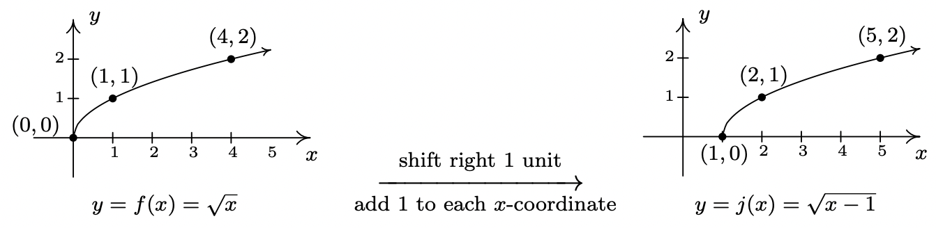
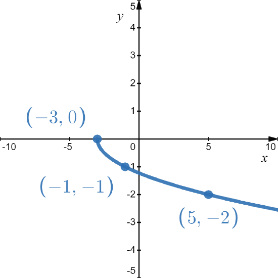
- To find the domain of \(m\), we solve \(x+3 \geq 0\) and get \([-3, \infty)\).
We have arrived at an example involving more than one transformation. Applying the Order of Transformations, the addition of \( 3 \) to \( x \) shifts the graph left \( 3 \) units. Hence, we subtract \(3\) from each of the \(x\)-coordinates of the points on the graph of \(f\) and arrive at our "stop-over" graph of \( m_1(x) \).
Applying the subtraction of \( 2 \) to the function value, we obtain the graph of \(m\) by subtracting \(2\) from the \(y\)-coordinates of each of the points on the graph of \(m_{1}(x)\). The resulting graph verifies that the domain of \(m\) is \([-3, \infty)\) and we find the range of \(m\) to be \([-2, \infty)\).
- Owing to the square root, the domain of \(f\) is \(x \geq 0\), or \([0,\infty)\).
Keep in mind that we can check our answer to any of these problems by showing that any of the points we've moved lie on the graph of our final answer. For example, we can check that \((-3,-2)\) is on the graph of \(m\) by computing \(m(-3) = \sqrt{(-3)+3} - 2 = \sqrt{0}-2 = -2. \checkmark\)
Reflections
At this point, we now know the effects of the parameters \( C \) and \( D \) on the graph of\[ h(x) = A f(Bx + C) + D. \nonumber \]In this subsection, we begin to look at the effects of the parameters of \( A \) and \( B \); however, we will only focus on their signs for the moment.
We know from Section 1.1 that to reflect a point \((x,y)\) across the \(x\)-axis, we replace \(y\) with \(-y\). If \((x_1,y_1)\) is on the graph of \(f\), then \(y_1=f(x_1)\), so replacing \(y_1\) with \(-y_1\) is the same as replacing \(f(x_1)\) with \(-f(x_1)\). Hence, the graph of \(y=-f(x)\) is the graph of \(f\) reflected across the \(x\)-axis. Similarly, the graph of \(y=f(-x)\) is the graph of \(f\) reflected across the \(y\)-axis.
Returning to the language of inputs and outputs, multiplying the output from a function by \(-1\) reflects its graph across the \(x\)-axis, while multiplying the input to a function by \(-1\) reflects the graph across the \(y\)-axis.
Suppose \(f\) is a function.
- The graph of \(y=-f(x)\) is obtained from reflecting the graph of \(y=f(x)\) across the \(x\)-axis by multiplying the \(y\)-coordinates of the points on the graph of \(f\) by \(-1\).
- The graph of \(y=f(-x)\) is obtained from reflecting the graph of \(y=f(x)\) across the \(y\)-axis by multiplying the \(x\)-coordinates of the points on the graph of \(f\) by \(-1\).
Applying this theorem to the graph of \(y=f(x)\) in Figure \( \PageIndex{1A} \), we can graph \(y=-f(x)\) by reflecting the graph of \(f\) about the \(x\)-axis (see Figure \( \PageIndex{5} \)).
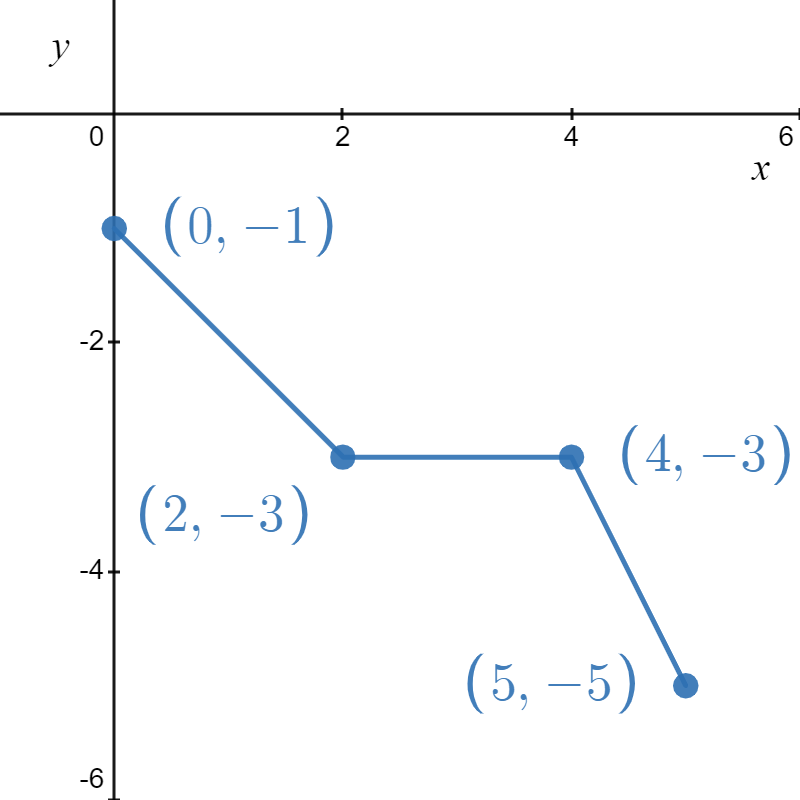
Figure \( \PageIndex{5} \): \( y = -f(x) \)
By reflecting the graph of \(f\) across the \(y\)-axis, we obtain the graph of \(y=f(-x)\) (see Figure \( \PageIndex{6} \)).
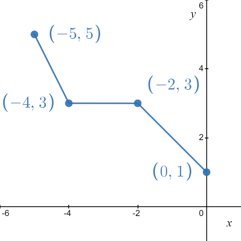
Figure \( \PageIndex{6} \): \( y = f(-x) \)
With the addition of reflections, considering the Order of Transformations is now more critical than ever, as we shall see in the following example. Remember, given\[ h(x) = A f(Bx + C) + D, \nonumber \]we will work from the "inside-out" following the Order of Operations.
Let \(f(x) = \sqrt{x}\). Use the graph of \(f\) in Figure \( \PageIndex{4} \) from Example \( \PageIndex{1} \) to graph the following functions. Also, state their domains and ranges.
- \(g(x) = \sqrt{-x}\)
- \(j(x) = \sqrt{3-x}\)
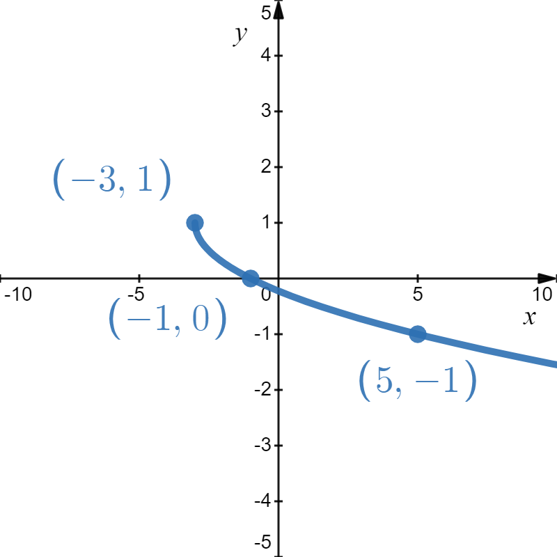
- \(m(x) = 3 - \sqrt{x}\)
- Solutions
-
- The mere sight of \(\sqrt{-x}\) usually causes alarm, if not panic. When we discussed domains in Section 1.4, we banished negatives from the radicands of even roots. However, we must remember that \(x\) is a variable, so the quantity \(-x\) isn't always negative. For example, if \(x=-4\), \(-x = 4\), thus \(\sqrt{-x} = \sqrt{-(-4)} = 2\) is perfectly well-defined. To find the domain analytically, we set \(-x \geq 0\) which gives \(x \leq 0\), so that the domain of \(g\) is \((-\infty, 0]\).
Since \(g(x) = f(-x)\), the reflection theorem tells us that the graph of \(g\) is the reflection of the graph of \(f\) across the \(y\)-axis. We accomplish this by multiplying each \(x\)-coordinate on the graph of \(f\) by \(-1\). Graphically, we see that the domain of \(g\) is \((-\infty, 0]\) and the range of \(g\) is the same as the range of \(f\), namely \([0,\infty)\).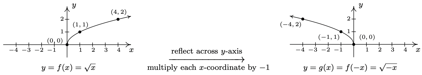
- To determine the domain of \(j(x) = \sqrt{3-x}\), we solve \(3-x \geq 0\) and get \(x \leq 3\), or \((-\infty, 3]\).
We have finally reached a point where Equation \ref{trans2} is critical to use. Many students will rewrite \( j(x) \) as \( j(x) = \sqrt{-x + 3} \). While this is correct, it's not enough because it does not showcase the correct horizontal shift. In the paragraph before Equation \ref{trans2}, we stated that \( C \) was being added to \( Bx \) - not \( x \). This is where factoring \( B \) in the argument of the function is necessary. According to the reflection theorem, a horizontal shift occurs when \( C \) is added to \( x \) - not \( Bx \)!
We start the graphing process by rewriting \( j(x) \) to match the form of Equation \ref{trans2}.\[ j(x) = \sqrt{3 - x} = \sqrt{-(-3 + x)} = \sqrt{-(x - 3)}. \nonumber \]Following the Order of Transformations, we first apply the transformation caused by the multiplication of \( -1 \) on \( x \). This will result in the "middleman" function, \( j_1(x) = \sqrt{-x} \). This reflects \( f \) about the \( y \)-axis.
Our next step in the Order of Transformations is to subtract \( 3 \) from \( x \) - not \( -x \) (again, this is why we needed to factor the argument). This shifts the graph of \( j_1 \) \( 3 \) units to the right. From the graph, we confirm the domain of \(j\) is \((-\infty, 3]\) and we get that the range is \([0, \infty)\).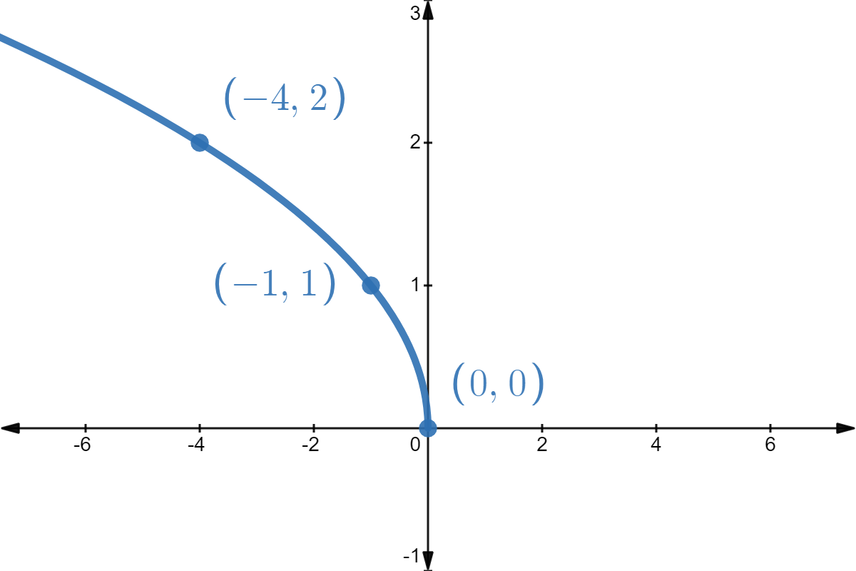
\( j_1(x) = \sqrt{-x} \)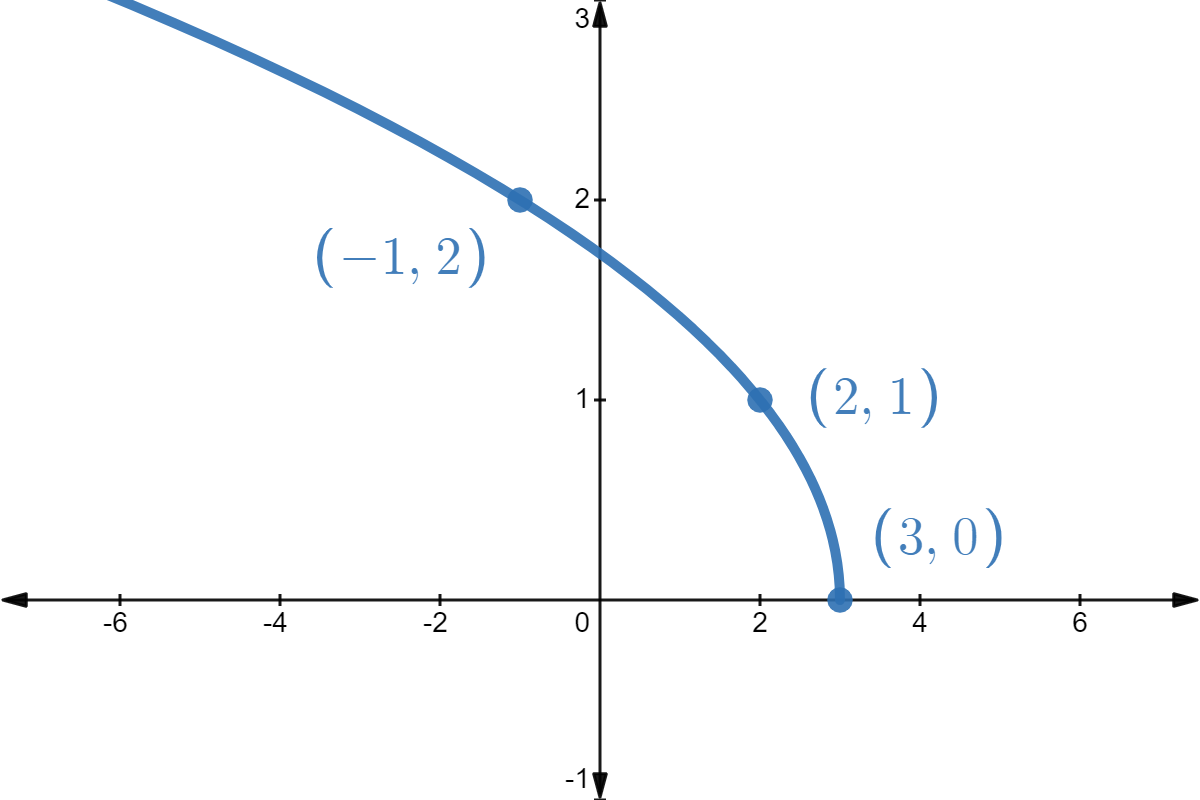
\( j(x) = \sqrt{-(x - 3)} \) - The domain of \(m\) works out to be the domain of \(f\), \([0, \infty)\).
Rewriting \(m(x) = -\sqrt{x} + 3\), we see \(m(x) = -f(x) + 3\). We perform a reflection across the \(x\)-axis using the Order of Transformations.
We then add \( 3 \) to the function values, which causes a shift up by \( 3 \) units. We see from the graph that the range of \(m\) is \((-\infty, 3]\).

- The mere sight of \(\sqrt{-x}\) usually causes alarm, if not panic. When we discussed domains in Section 1.4, we banished negatives from the radicands of even roots. However, we must remember that \(x\) is a variable, so the quantity \(-x\) isn't always negative. For example, if \(x=-4\), \(-x = 4\), thus \(\sqrt{-x} = \sqrt{-(-4)} = 2\) is perfectly well-defined. To find the domain analytically, we set \(-x \geq 0\) which gives \(x \leq 0\), so that the domain of \(g\) is \((-\infty, 0]\).
Vertical Scalings
We now turn our attention to our last class of transformations known as scalings. A thorough discussion of scalings can get complicated because they are not as straightforward as the previous transformations. A quick review of what we've covered so far, namely vertical shifts, horizontal shifts, and reflections, will show you why those transformations are known as rigid transformations. Simply put, they do not change the shape of the graph, only its position and orientation in the plane. If, however, we wanted to make a new graph twice as tall as a given graph or one-third as wide, we would be changing the shape of the graph. This type of transformation is called non-rigid for obvious reasons. Not only will it be important for us to differentiate between modifying inputs versus outputs, but we must also pay close attention to the magnitude of the changes we make. As you will see, the Mathematics is easier than the associated grammar.
Suppose we wish to graph the function \(h(x) =2 f(x)\) where \(f(x)\) is the function from Figure \( \PageIndex{1A} \) given at the beginning of the section. From its graph, we can build a table of values for \(h\) as before.\[\begin{array}{|c|c|c|}
\hline x & f(x) & h(x)=2f(x) \\
\hline 0 & 1 & 2 \\
\hline 2 & 3 & 6 \\
\hline 4 & 3 & 6 \\
\hline 5 & 5 & 10 \\
\hline \end{array} \nonumber \]In general, if \((x_1,y_1)\) is on the graph of \(f\), then \(f(x_1) = y_1\) so that \(h(x_1) = 2 f(x_1) = 2y_1\) puts \((x_1,2y_1)\) on the graph of \(h\). In other words, to obtain the graph of \(h\), we multiply all of the \(y\)-coordinates of the points on the graph of \(f\) by \(2\). Multiplying all of the \(y\)-coordinates of all of the points on the graph of \(f\) by \(2\) causes what is known as a vertical scaling (also called a vertical stretching, vertical expansion, or vertical dilation) by a factor of \(2\), and the results are shown below.

If we wish to graph \(y = \frac{1}{2} g(x)\), where \( g(x) \) is from Figure \( \PageIndex{1B} \), we multiply the all of the \(y\)-coordinates of the points on the graph of \(g\) by \(\frac{1}{2}\). This creates a vertical compression (also called vertical shrinking or vertical contraction) by a factor of \(2\) as seen below.
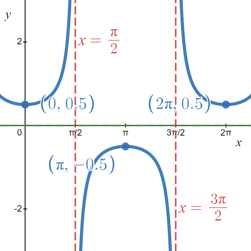
Figure \( \PageIndex{7} \): \( h(x) = \frac{1}{2} \sec{(x)} \)
These results are generalized in the following theorem.
Suppose \(f\) is a function and \(a \gt 0\). The graph of \(y=a f(x)\) is obtained by multiplying all of the \(y\)-coordinates of the points on the graph of \(f\) by \(a\). We say the graph of \(f\) has been vertically scaled by a factor of \(a\).
- If \(a > 1\), we say the graph of \(f\) has undergone a vertical stretching (expansion, dilation) by a factor of \(a\).
- If \(0 < a < 1\), we say the graph of \(f\) has undergone a vertical shrinking (compression, contraction) by a factor of \(\frac{1}{a}\).
A few remarks about this theorem are in order. First, a note about the vocabulary. To the authors, the words "stretching," "expansion," and "dilation" all indicate something getting bigger. Hence, "stretched by a factor of \(2\)" makes sense if we are scaling something by multiplying it by \(2\).
Similarly, we believe words like "shrinking," "compression," and "contraction" all indicate something getting smaller, so if we scale something by a factor of \(\frac{1}{2}\), we would say it "shrinks by a factor of \(2\)" - not "shrinks by a factor of \(\frac{1}{2}\)." This is why we have written the descriptions "stretching by a factor of \(a\)" and "shrinking by a factor of \(\frac{1}{a}\)" in the statement of the theorem.
Second, in terms of inputs and outputs, this theorem says multiplying the outputs from a function by positive number \(a\) causes the graph to be vertically scaled by a factor of \(a\). It is natural to ask what would happen if we multiply a function's inputs by a positive number. This leads us to our last transformation of the section.
Finally, returning to the Order of Transformations, we now understand the role of \( A \) in\[ h(x) = A f(Bx + C) + D. \nonumber \]So far, when applying transformations, we do the following:
- Multiply \( x \) by \( B \) to get ???
- Add \( C \) to \( x \) to shift the graph horizontally.
- Multiply the function values by \( A \) to possibly reflect the graph about the \( x \)-axis, and stretch or compress the graph vertically (away from the \( x \)-axis).
- Add \( D \) to the function values to shift the graph vertically.
Horizontal Scalings
Again, referring to the graph of \(f\) in Figure \( \PageIndex{1A} \), suppose we want to graph \(h(x) = f(2x)\). In other words, we are looking to see what effect multiplying the inputs to \(f\) by \(2\) has on its graph. Suppose we attempt to build a table directly. In that case, we quickly run into the same problem we had in our discussion leading up to the theorem on horizontal shifts, as seen in the table below.\[\begin{array}{|c|c|c|}
\hline x & f(x) & h(x)=f(2 x) \\
\hline 0 & 1 & f(2 \cdot 0)=f(0)=1\\
\hline 2 & 3 & f(2 \cdot 2)=f(4)=3 \\
\hline 4 & 3 & f(2 \cdot 4)=f(8)=? \\
\hline 5 & 5 & f(2 \cdot 5)=f(10)=? \\
\hline
\end{array}\nonumber \]We solve this problem in the same way we solved this problem before. For example, if we want to determine the point on \(h\) which corresponds to the point \((2,3)\) on the graph of \(f\), we set \(2x =2\) so that \(x=1\). Substituting \(x=1\) into \(h(x)\), we obtain \(h(1) = f(2 \cdot 1) = f(2) = 3\), so that \((1,3)\) is on the graph of \(h\). Continuing in this fashion, we obtain the table below.\[ \begin{array}{|c|c|c|}
\hline x & 2 x & h(x)=f(2 x) \\
\hline 0 & 0 & h(0)=f(0)=1 \\
\hline 1 & 2 & h(1)=f(2)=3 \\
\hline 2 & 4 & h(2)=f(4)=3 \\
\hline \dfrac{5}{2} & 5 & h\left(\dfrac{5}{2}\right)=f(5)=5 \\
\hline
\end{array} \nonumber \]In general, if \((x_1,y_1)\) is on the graph of \(f\), then \(f(x_1) = y_1\). Hence \(h\left(\frac{x_1}{2}\right) = f\left(2 \cdot \frac{x_1}{2}\right) = f(x_1) = y_1\) so that \(\left(\frac{x_1}{2}, y_1\right)\) is on the graph of \(h\).
In other words, to graph \(h\) we divide the \(x\)-coordinates of the points on the graph of \(f\) by \(2\). This results in a horizontal scaling (also called horizontal shrinking, horizontal compression, or horizontal contraction) by a factor of \(\frac{1}{2}\).

If, on the other hand, we wish to graph \(y = g\left( \frac{1}{2} x\right)\) from Figure \( \PageIndex{1B} \), we end up multiplying the \(x\)-coordinates of the points on the graph of \(g\) by \(2\) which results in a horizontal scaling (also called horizontal stretching, horizontal expansion, or horizontal dilation) by a factor of \(2\), as demonstrated below.
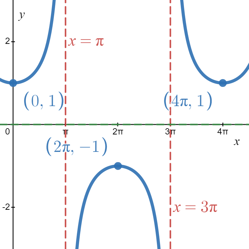
Figure \( \PageIndex{8} \): \( h(x) = \sec{\left( \frac{1}{2} x \right)} \)
It is instructive to note that in Figure \( \PageIndex{8} \), we have not only multiplied the \( x \)-values of our anchor points by \( 2 \) but also the values of the vertical asymptotes by \( 2 \) as well.
We have the following theorem.
Suppose \(f\) is a function and \(b>0\). The graph of \(y= f(bx)\) is obtained from dividing all of the \(x\)-coordinates of the points on the graph of \(f\) by \(b\). We say the graph of \(f\) has been horizontally scaled by a factor of \(\frac{1}{b}\).
- If \(0 < b < 1\), we say the graph of \(f\) has undergone a horizontal stretching (expansion, dilation) by a factor of \(\frac{1}{b}\).
- If \(b>1\), we say the graph of \(f\) has undergone a horizontal shrinking (compression, contraction) by a factor of \(b\).
This theorem tells us that if we multiply the input to a function by \(b\), the resulting graph is scaled horizontally by a factor of \(\frac{1}{b}\) since the \(x\)-values are divided by \(b\) to produce corresponding points on the graph of \(y = f(bx)\).
The next example explores how vertical and horizontal scalings sometimes interact with each other and with the other transformations introduced in this section.
Let \(f(x)= \sqrt{x}\). Use the graph of \(f\) from Figure \( \PageIndex{4} \) in Example \( \PageIndex{1} \) to graph the following functions. Also, state their domains and ranges.
- \(g(x) = 3 \sqrt{x}\)
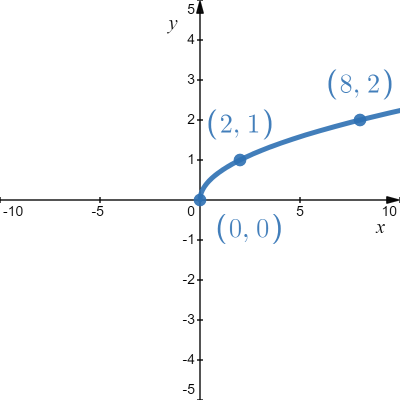
- \(j(x) = \sqrt{9x}\)
- \(m(x) =1 - \sqrt{\frac{x+3}{2}}\)
- Solutions
-
- First we note that the domain of \(g\) is \([0, \infty)\) for the usual reason.
Next, we have \(g(x) = 3 f(x)\). So, we obtain the graph of \(g\) by multiplying all of the \(y\)-coordinates of the points on the graph of \(f\) by \(3\). The result is a vertical scaling of the graph of \(f\) by a factor of \(3\). We find the range of \(g\) is also \([0, \infty)\).
- To determine the domain of \(j\), we solve \(9x \geq 0\) to find \(x \geq 0\). Again, Our domain is \([0,\infty)\).
We recognize \(j(x) = f(9x)\) and by our most recent theorem, we obtain the graph of \(j\) by dividing the \(x\)-coordinates of the points on the graph of \(f\) by \(9\). From the graph, we see the range of \(j\) is also \([0,\infty)\).
- This is the whole enchilada. It has most of the transformations, so we have to be very meticulous with our work. As usual, let's start by finding the domain. Solving \(\frac{x+3}{2} \geq 0\) gives \(x \geq -3\), so the domain of \(m\) is \([-3, \infty)\).
To take advantage of the Order of Transformations, we rewrite \[m(x) = - \sqrt{\dfrac{1}{2} x + \dfrac{3}{2}} + 1 = - \sqrt{\dfrac{1}{2} \left(x + 3\right)} + 1.\nonumber\]- The coefficient of \( x \) prior to factoring is \( \frac{1}{2} \). This will cause a horizontal stretch by a factor of 2.
- Once we factored the \( \frac{1}{2} \) from the argument \( \frac{1}{2} x + \frac{3}{2} \), the true horizontal shift is revealed. Remember, the addition or subtraction of \( C \) from \( x \) represents the horizontal shift - not the addition or subtraction of \( C \) from \( Bx \). Since \( B \left( x + \frac{C}{B} \right) = \frac{1}{2} \left( x + 3 \right) \), the graph experiences a horizontal shift to the left two units.
- The coefficient of the function is negative. Hence, the graph gets reflected about the \( x \)-axis; however, there is no additional vertical scaling because \( | - 1 | = 1 \).
- Finally, the addition of 1 to the function values shifts the graph up 1 unit.


Left: \( f(x) = \sqrt{x} \) and Right: \( m_1(x) = \sqrt{\frac{1}{2} x} \)
Left: \( m_2(x) = \sqrt{\frac{1}{2}(x + 3)} \) and Right: \( m_3(x) = -\sqrt{\frac{1}{2} \left(x + 3\right)} \)
\( m(x) = -\sqrt{\frac{1}{2} \left(x + 3\right)} + 1 \) - First we note that the domain of \(g\) is \([0, \infty)\) for the usual reason.

Note, recalling the properties of radicals from Intermediate Algebra, we know that the functions \(g\) and \(j\) are the same, since \(j\) and \(g\) have the same domains and \(j(x) = \sqrt{9x} = \sqrt{9} \sqrt{x} = 3 \sqrt{x} = g(x)\). (We invite the reader to verify that all of the points we plotted on the graph of \(g\) lie on the graph of \(j\) and vice-versa.) Hence, for \(f(x) = \sqrt{x}\), a vertical stretch by a factor of \(3\) and a horizontal shrinking by a factor of \(9\) result in the same transformation. While this kind of phenomenon is not universal, it happens commonly enough with some of the families of functions studied in College Algebra that it is worthy of note.
Below is the complete graph of \(y = f(x)\). Use it to graph \(g(x) = \frac{4-3 f(1-2x)}{2}\).

- Solution
-
We first rewrite \( g \) in the form of Equation \ref{trans2}.\[ g(x) = -\frac{3}{2} f\left( -2\left(x - \frac{1}{2} \right)\right) + 2. \nonumber \]From the Order of Transformations, we have the following:\[ \begin{array}{|c|c|c|c|c|c|c|}
\hline \text{Current} & \text{Transformation} & \text{Anchor Point} & \text{Anchor Point} & \text{Anchor Point} & \text{Anchor Point} & \text{Anchor Point} \\
\text{Function} & & (-4,-3) & (-2,0) & (0,3) & (2,0) & (4,-3) \\
\hline f(-x) & \text{reflection about the }y\text{-axis} & (4,-3) & (2,0) & (0,3) & (-2,0) & (-4,-3) \\
\hline f(-2x) & \text{horizontal compression by a factor of }\frac{1}{2} & \left(2,-3\right) & \left(1,0\right) & \left(0,3\right) & \left(-1,0\right) & \left(-2,-3\right) \\
\hline f(-2\left(x - \frac{1}{2}\right)) & \text{horizontal shift right by }\frac{1}{2}\text{ unit} & \left(\frac{5}{2},-3\right) & \left(\frac{3}{2},0\right) & \left(\frac{1}{2},3\right) & \left(-\frac{1}{2},0\right) & \left(-\frac{3}{2},-3\right) \\
\hline -f(-2\left(x - \frac{1}{2}\right)) & \text{reflection about }x\text{-axis} & \left(\frac{5}{2},3\right) & \left(\frac{3}{2},0\right) & \left(\frac{1}{2},-3\right) & \left(-\frac{1}{2},0\right) & \left(-\frac{3}{2},3\right) \\
\hline -\frac{3}{2}f(-2\left(x - \frac{1}{2}\right)) & \text{vertical stretch by a factor of }\frac{3}{2} & \left(\frac{5}{2},\frac{9}{2}\right) & \left(\frac{3}{2},0\right) & \left(\frac{1}{2},-\frac{9}{2}\right) & \left(-\frac{1}{2},0\right) & \left(-\frac{3}{2},\frac{9}{2}\right) \\
\hline -\frac{3}{2}f(-2\left(x - \frac{1}{2}\right)) + 2 & \text{vertical shift up by }2\text{ units} & \left(\frac{5}{2},\frac{13}{2}\right) & \left(\frac{3}{2},2\right) & \left(\frac{1}{2},-\frac{5}{2}\right) & \left(-\frac{1}{2},2\right) & \left(-\frac{3}{2},\frac{13}{2}\right) \\
\hline \end{array} \nonumber \]To graph \(g\), we plot each of the points in the table above and connect them in the same order and fashion as the points to which they correspond. Plotting \(f\) and \(g\) side-by-side gives
The reader is strongly encouraged to graph the series of functions, which shows the gradual transformation of the graph of \(f\) into the graph of \(g\). We have outlined the sequence of transformations in the above exposition; all that remains is to plot the five intermediate stages.
The Order of Transformations
We finish this section with the cleaned-up version of the Order of Transformations.
Let \( h(x) \) be a function that can be written as\[ h(x) = A f(Bx + C) + D = A f\left(B \left( x + \frac{C}{B} \right) \right) + D, \nonumber \]for constants \( A \), \( B \), \( C \), and \( D \), where \( A \neq 0 \) and \( B \neq 0 \). The graph of \( h \) can be obtained from the graph of \( f \) as follows:
- Start with the base graph, \( f(x) \).
- If \( B \lt 0 \), horizontally reflect the graph about the \( y \)-axis.
- If \( 0 \lt |B| \lt 1 \), horizontally stretch the graph by a factor of \( \frac{1}{B} \). Otherwise, if \( |B| \gt 1 \), horizontally compress the graph by a factor of \( B \).
- Horizontally shift the graph \(\frac{C}{B}\) units to the left (if \(\frac{C}{B} \gt 0\)) or right (if \(\frac{C}{B} \lt 0\)).
-
- If \( A \lt 0 \), vertically reflect the graph about the \( x \)-axis.
- If \( |A| \gt 1 \), vertically stretch the graph by a factor of \( A \). Otherwise, if \( 0 \lt |A| \lt 1 \), vertically compress the graph by a factor of \( \frac{1}{A} \).
- Vertically shift the graph \( D \) units up (if \( D \gt 0 \)) or down (if \( D \lt 0 \)).
Footnotes
1 In reality, the Fundamental Graphing Principle for Functions states for a point \( \left( x,y \right) \) to be on the graph, \( f(x) = y \); however, I personally find that replacing \( x \) and \( y \) with \( x_1 \) and \( y_1 \), respectively, makes the language a little more understandable.
2 An "anchor point" is a point on a base graph that you "track" as you perform transformations.
3 There is no real need to know what the secant function is at this point - don't worry.
4 In reality, we are performing the Order of Operations in alphabetical order. We first focus on what happens to the \( x \) values, then what happens to the \( y \) values, which are the function values.
5 If this was truly the Order of Operations, at this point we would apply the function \( f \) to the argument \( Bx + C \); however, we will not need to do that in the graphing process. You will just have to wait and see why.
6 This order is flexible and, in practice, most people perform it from \( A \) to \( D \).
7 The word "better" here is debatable. Since these equations are equivalent, one is not technically "better" than the other. However, for our conversation and the way I am presenting this topic, Equation \ref{trans2} is more convenient.
8 For those "in the know," this terminology ("standard form" versus "general form") aligns nicely with all related definitions of standard and general forms you will see in Mathematics. Generally, an equation in standard form is a factored form, and an equation in general form is a distributed form.
9 Truth be told, horizontal and vertical shifts can be applied in either order; however, I will stick with the convention listed in the Order of Transformations.