6.5: Applications of Exponential and Logarithmic Functions

Math 370 Learning Objectives

• Analyze and model financial problems involving continuous compounding.
• Understand and use relative growth rates in population models.
• Use half-life to model decay problems.
• Use Newton's Law of Cooling and logistic growth models.

As we mentioned in Section 6.1, exponential and logarithmic functions are used to model a wide variety of behaviors in the real world. In the examples that follow, note that while the applications are drawn from many different disciplines, the mathematics remains essentially the same. Due to the applied nature of the problems we will examine in this section, the calculator is often used to express our answers as decimal approximations.

---

Applications of Exponential Functions

Financial Models

Perhaps the most well-known application of exponential functions comes from the financial world. Suppose you have \(\$ 100\) to invest at your local bank and they are offering a whopping \(5 \, \%\) annual percentage interest rate. This means that after one year, the bank will pay you \(5 \%\) of that \(\$100\), or \(\$ 100(0.05) =\$ 5\) in interest, so you now have \(\$105\). This is in accordance with the formula for simple interest which you have undoubtedly run across at some point before.

Theorem \(\PageIndex{1}\): Simple Interest

The amount of interest \(I\) accrued at an annual rate \(r\) on an investment¹ \(P_0\) (pronounced "\( P \) nought") after \(t\) years is \[I = P_0 rt. \nonumber\]The amount \(A\) in the account after \(t\) years is given by \[A = P_0 + I = P_0 + P_0rt = P_0(1+rt).\nonumber\]

Suppose, however, that six months into the year, you hear of a better deal at a rival bank. Naturally, you withdraw your money and try to invest it at the higher rate there. Since six months is one half of a year, that initial \(\$100\) yields \(\$100(0.05)\left(\frac{1}{2}\right) = \$ 2.50\) in interest. You take your \(\$102.50\) off to the competitor and find out that those restrictions which may apply actually apply to you, and you return to your bank which happily accepts your \(\$102.50\) for the remaining six months of the year.

To your surprise and delight, at the end of the year your statement reads \(\$105.06\), not \(\$105\) as you had expected.² Where did those extra six cents come from? For the first six months of the year, interest was earned on the original principal of \(\$100\), but for the second six months, interest was earned on \(\$102.50\), that is, you earned interest on your interest.

This is the basic concept behind compound interest. In the previous discussion, we would say that the interest was compounded twice, or semiannually.³ If more money can be earned by earning interest on interest already earned, a natural question to ask is what happens if the interest is compounded more often, say \(4\) times a year, which is every three months, or "quarterly." In this case, the money is in the account for three months, or \(\frac{1}{4}\) of a year, at a time. After the first quarter, we have \[A = P_0(1+rt) = \$100 \left(1 + 0.05 \cdot \dfrac{1}{4} \right) = \$101.25. \nonumber\]We now invest the \(\$101.25\) for the next three months and find that at the end of the second quarter, we have \[A = \$101.25 \left(1 + 0.05 \cdot \dfrac{1}{4} \right)\approx \$102.51.\nonumber\]Continuing in this manner, the balance at the end of the third quarter is \(\$103.79\), and, at last, we obtain \(\$105.08\). The extra two cents hardly seems worth it, but we see that we do in fact get more money the more often we compound.

In order to develop a formula for this phenomenon, we need to do some abstract calculations. Suppose we wish to invest our principal \(P_0\) at an annual rate \(r\) and compound the interest \(n\) times per year. This means the money sits in the account \(\frac{1}{n}^{\text{th}}\) of a year between compoundings. Let \(A_{k}\) denote the amount in the account after the \(k^{\text{th}}\) compounding. Then \[A_{1} = P_0\left(1 + r\left(\dfrac{1}{n}\right)\right),\nonumber\]which simplifies to \[A_{1} = P_0 \left(1 + \dfrac{r}{n}\right).\nonumber\]After the second compounding, we use \(A_{1}\) as our new principal and get \[A_{2} = A_{1} \left(1 + \dfrac{r}{n}\right) = \left[P_0 \left(1 + \dfrac{r}{n}\right)\right]\left(1 + \dfrac{r}{n}\right) = P_0 \left(1 + \dfrac{r}{n}\right)^2.\nonumber\]Continuing in this fashion, we get \[A_{3} =P_0 \left(1 + \dfrac{r}{n}\right)^3, A_{4} =P_0 \left(1 + \dfrac{r}{n}\right)^4,\nonumber\]and so on, so that \[A_{k} = P_0 \left(1 + \dfrac{r}{n}\right)^k.\nonumber\]Since we compound the interest \(n\) times per year, after \(t\) years, we have \(nt\) compoundings. We have just derived the general formula for compound interest below.

Theorem \(\PageIndex{2}\): Compound Interest

If an initial principal \(P_0\) is invested at an annual rate \(r\) and the interest is compounded \(n\) times per year, the amount \(A\) in the account after \(t\) years is \[A(t) = P_0 \left(1 + \dfrac{r}{n}\right)^{nt}.\nonumber\]

If we take \(P_0 = 100\), \(r = 0.05\), and \(n = 4\), then we have \(A(t) = 100\left(1+ \frac{0.05}{4}\right)^{4t}\) which reduces to \(A(t) = 100(1.0125)^{4t}\). To check this new formula against our previous calculations, we find \(A\left(\frac{1}{4}\right) = 100(1.0125)^{4 \left(\frac{1}{4}\right)} = 101.25\), \(A\left(\frac{1}{2}\right) \approx \$102.51\), \(A\left(\frac{3}{4}\right) \approx \$103.79\), and \(A(1) \approx \$105.08\).

Example \( \PageIndex{1} \)

Suppose \(\$2000\) is invested in an account which offers \(7.125 \%\) compounded monthly.

1. Express the amount \(A\) in the account as a function of the term of the investment \(t\) in years.
2. How much is in the account after \(5\) years?
3. How long will it take for the initial investment to double?
4. Find and interpret the average rate of change⁴ of the amount in the account from the end of the fourth year to the end of the fifth year, and from the end of the thirty-fourth year to the end of the thirty-fifth year.

Solution

1. Substituting \(P_0 = 2000\), \(r = 0.07125\), and \(n = 12\) (since interest is compounded monthly) into the compound interest formula yields \(A(t) = 2000\left(1 + \frac{0.07125}{12}\right)^{12t}=2000 (1.0059375)^{12t}\).
2. Since \(t\) represents the length of the investment in years, we substitute \(t=5\) into \(A(t)\) to find \(A(5) = 2000 (1.0059375)^{12(5)} \approx 2852.92\). After \(5\) years, we have approximately \(\$2852.92\).
3. Our initial investment is \(\$2000\), so to find the time it takes this to double, we need to find \(t\) when \(A(t) = 4000\). We get \(2000 (1.0059375)^{12t}=4000\), or \((1.0059375)^{12t}=2\). Taking natural logs as in Section 6.3, we get \(t = \frac{\ln(2)}{12 \ln(1.0059375)} \approx 9.75\). Hence, it takes approximately \(9\) years \(9\) months for the investment to double.
4. To find the average rate of change of \(A\) from the end of the fourth year to the end of the fifth year, we compute \(\frac{A(5)-A(4)}{5-4} \approx 195.63\). Similarly, the average rate of change of \(A\) from the end of the thirty-fourth year to the end of the thirty-fifth year is \(\frac{A(35)-A(34)}{35-34} \approx 1648.21\). This means that the value of the investment is increasing at a rate of approximately \(\$195.63\) per year between the end of the fourth and fifth years, while that rate jumps to \(\$1648.21\) per year between the end of the thirty-fourth and thirty-fifth years. So, not only is it true that the longer you wait, the more money you have, but also the longer you wait, the faster the money increases.⁵

We have observed that the more times you compound the interest per year, the more money you will earn in a year. Let’s push this notion to the limit.⁶ Consider an investment of \(\$ 1\) invested at \(100 \%\) interest for \(1\) year compounded \(n\) times a year. The compound interest formula tells us that the amount of money in the account after \(1\) year is \(A = \left(1+\frac{1}{n}\right)^{n}\). Below is a table of values relating \(n\) and \(A\).

\[\begin{array}{|r||r|} \hline n & A \\ \hline 1 & 2 \\ \hline 2 & 2.25 \\ \hline 4 & \approx 2.4414 \\ \hline 12 & \approx 2.6130 \\ \hline 360 & \approx 2.7145 \\ \hline 1000 & \approx 2.7169 \\ \hline 10000 & \approx 2.7181 \\ \hline 100000 & \approx 2.7182 \\ \hline \end{array}\nonumber\]

As promised, the more compoundings per year, the more money there is in the account, but we also observe that the increase in money is greatly diminishing. We are witnessing a mathematical "tug of war." While we are compounding more times per year, and hence getting interest on our interest more often, the amount of time between compoundings is getting smaller and smaller, so there is less time to build up additional interest. With Calculus, we can show⁷ that as \(n \to \infty\), \(A = \left(1+\frac{1}{n}\right)^{n} \to e\), where \(e\) is the natural base first presented in Section 6.1. Taking the number of compoundings per year to infinity results in what is called continuously compounded interest.

Theorem \(\PageIndex{3}\)

If you invest \(\$1\) at \(100 \%\) interest compounded continuously, then you will have \(\$ e\) at the end of one year.

Using this definition of \(e\) and a little Calculus, we can take the compound interest formula and produce a formula for continuously compounded interest.

Theorem \(\PageIndex{4}\): Continuously Compounded Interest

If an initial principal \(P_0\) is invested at an annual rate \(r\) and the interest is compounded continuously, the amount \(A\) in the account after \(t\) years is \[A(t) = P_0 e^{rt}.\nonumber\]

If we take the scenario of Example \( \PageIndex{1} \) and compare monthly compounding to continuous compounding over \(35\) years, we find that monthly compounding yields \(A(35) = 2000 (1.0059375)^{12(35)}\) which is about \(\$ 24,\!035.28\), whereas continuously compounding gives \(A(35) = 2000e^{0.07125 (35)}\) which is about \(\$ 24,\!213.18\) - a difference of less than \(1 \%\).

Subsection Footnotes

¹ Called the principal.

² Actually, the final balance should be $105.0625.

³ Using this convention, simple interest after one year is the same as compounding the interest only once.

⁴ See Section 2.1 for the definition of the average rate of change.

⁵ In fact, the rate of increase of the amount in the account is exponential as well. This is the quality that really defines exponential functions and we refer the reader to a course in Calculus.

⁶ Once you’ve had a semester of Calculus, you’ll be able to fully appreciate this very lame pun.

⁷ Or define, depending on your point of view.

Population Growth Models

The compound interest and continuously compounding interest formulas both use exponential functions to describe the growth of an investment. Curiously enough, the same principles which govern compound interest are also used to model short term growth of populations. In Biology, The Law of Uninhibited Growth states as its premise that the instantaneous rate at which a population increases at any time is directly proportional to the population at that time.⁸ In other words, the more organisms there are at a given moment, the faster they reproduce. Formulating the law as stated results in a differential equation, which requires Calculus to solve. Its solution is stated below.

Theorem \(\PageIndex{5}\): Uninhibited Growth

If a population increases according to The Law of Uninhibited Growth, the population of organisms \(P\) at time \(t\) is given by the formula \[P(t) = P_0e^{rt},\nonumber\]where \(P(0) = P_0\) is the initial number of organisms and \(r>0\) is the constant of proportionality which satisfies the equation \[\text{instantaneous rate of change of }P(t)\text{ at time }t = r \, P(t).\nonumber\]

It is worth taking some time to compare the formulas for continuously compounding interest and the equation of uninhibited growth. In continuous compounding, we use \(P_0\) to denote the initial investment. In the formula for uninhibited growth, we use \(P_0\) to denote the initial population. In the continuous compounding formula, \(r\) denotes the annual interest rate, and so it shouldn’t be too surprising that the \(r\) in the uninhibited growth formula corresponds to a growth rate as well.

Example \( \PageIndex{2} \)

In order to perform arthrosclerosis research, epithelial cells are harvested from discarded umbilical tissue and grown in the laboratory. A technician observes that a culture of twelve thousand cells grows to five million cells in one week. Assuming that the cells follow The Law of Uninhibited Growth, find a formula for the number of cells, \(P\), in thousands, after \(t\) days.

Solution

We begin with \(P(t) = P_0e^{rt}\). Since \(P\) is to give the number of cells in thousands, we have \(P_0 = 12\), so \(P(t) = 12e^{rt}\). In order to complete the formula, we need to determine the growth rate \(r\). We know that after one week, the number of cells has grown to five million. Since \(t\) measures days and the units of \(P\) are in thousands, this translates mathematically to \(P(7) = 5000\). We get the equation \(12e^{7r} = 5000\) which gives \(r = \frac{1}{7} \ln\left(\frac{1250}{3}\right)\). Hence, \(P(t) = 12e^{ \frac{t}{7} \ln\left(\frac{1250}{3}\right)}\). Of course, in practice, we would approximate \(r\) to some desired accuracy, say \(r \approx 0.8618\), which we can interpret as an \(86.18 \%\) daily growth rate for the cells.

Subsection Footnotes

⁸ The average rate of change of a function over an interval was first introduced in Section 2.1. Instantaneous rates of change are the business of Calculus.

Population Decay Models

Whereas the formulas for continuous compounding and uninhibited growth model the growth of quantities, we can use equations like them to describe the decline of quantities. One example we’ve seen already is Example 6.1.1 in Section 6.1. There, the value of a car declined from its purchase price of \(\$25,\!000\) to nothing at all. Another real world phenomenon which follows suit is radioactive decay. There are elements which are unstable and emit energy spontaneously. In doing so, the amount of the element itself diminishes. The assumption behind this model is that the rate of decay of an element at a particular time is directly proportional to the amount of the element present at that time. In other words, the more of the element there is, the faster the element decays. This is precisely the same kind of hypothesis which drives The Law of Uninhibited Growth, and as such, the equation governing radioactive decay is hauntingly similar to the formula for uninhibited growth with the exception that the rate constant \(r\) is negative.

Theorem \(\PageIndex{6}\): Radioactive Decay

The amount of a radioactive element \(P\)⁹ at time \(t\) is given by the formula \[P(t) = P_0e^{rt},\nonumber\]where \(P(0) = P_0\) is the initial amount of the element and \(r<0\) is the constant of proportionality which satisfies the equation

\[\text{instantaneous rate of change of }P(t)\text{ at time }t = r \, P(t).\nonumber\]

Example \( \PageIndex{3} \)

Iodine-131 is a commonly used radioactive isotope used to help detect how well the thyroid is functioning. Suppose the decay of Iodine-131 follows the radioactive decay model, and that the half-life¹⁰ of Iodine-131 is approximately \(8\) days. If \(5\) grams of Iodine-131 is present initially, find a function which gives the amount of Iodine-131, \(A\), in grams, \(t\) days later.

Solution

Since we start with \(5\) grams initially, our initial formula is \(P(t) = 5e^{rt}\). Since the half-life is \(8\) days, it takes \(8\) days for half of the Iodine-131 to decay, leaving half of it behind. Hence, \(P(8) = 2.5\) which means \(5e^{8r} = 2.5\). Solving, we get \(r = \frac{1}{8} \ln\left(\frac{1}{2}\right) = -\frac{\ln(2)}{8} \approx -0.08664\), which we can interpret as a loss of material at a rate of \(8.664 \%\) daily. Hence, \[P(t) = 5 e^{-\frac{t\ln(2)}{8}} \approx 5 e^{-0.08664t}.\nonumber\]

Subsection Footnotes

⁹ If you haven't figured it our by now, we use \( P \) for the dependent variable and \( P_0 \) for \( P(0) \) because almost all exponential models can be thought of as modeling a population \( P \) that starts with a "time zero" population (a.k.a., an initial population) of \( P_0 \).

¹⁰ The time it takes for half of the substance to decay.

Newton's Law of Cooling

We now turn our attention to some more mathematically sophisticated models. One such model is Newton’s Law of Cooling, which we first encountered in Example 6.1.2 of Section 6.1. In that example we had a cup of coffee cooling from \(160^{\circ}\text{F}\) to room temperature \(70^{\circ}\text{F}\) according to the formula \(T(t) = 70 + 90 e^{-0.1 t}\), where \(t\) was measured in minutes. In this situation, we know the physical limit of the temperature of the coffee is room temperature,¹¹ and the differential equation which gives rise to our formula for \(T(t)\) takes this into account.

Whereas the radioactive decay model had a rate of decay at time \(t\) directly proportional to the amount of the element which remained at time \(t\), Newton’s Law of Cooling states that the rate of cooling of the coffee at a given time \(t\) is directly proportional to how much of a temperature differential exists between the coffee at time \(t\) and room temperature, not the temperature of the coffee itself. In other words, the coffee cools faster when it is first served, and as its temperature nears room temperature, the coffee cools ever more slowly. Of course, if we take an item from the refrigerator and let it sit out in the kitchen, the object’s temperature will rise to room temperature, and since the physics behind warming and cooling is the same, we combine both cases in the equation below.

Theorem \(\PageIndex{7}\): Newton's Law of Cooling (and Warming)

The temperature \(T\) of an object at time \(t\) is given by the formula \[T(t) = T_{a} + \left(T_0 - T_{a}\right) e^{-kt},\nonumber\]where \(T(0) = T_0\) is the initial temperature of the object, \(T_{a}\) is the ambient temperature¹² and \(k>0\) is the constant of proportionality which satisfies the equation \[\text{instantaneous rate of change of }T(t)\text{ at time }t = k \, \left(T(t) - T_{a}\right)\nonumber\]

If we re-examine the situation in Example 6.1.2 with \(T_0 = 160\), \(T_{a} = 70\), and \(k = 0.1\), we get, according to Newton's Law of Cooling, \(T(t) = 70 + (160 - 70)e^{-0.1t}\) which reduces to the original formula given. The rate constant \(k = 0.1\) indicates the coffee is cooling at a rate equal to \(10 \%\) of the difference between the temperature of the coffee and its surroundings. Note in Newton's Law of Cooling that the constant \(k\) is positive for both the cooling and warming scenarios. What determines if the function \(T(t)\) is increasing or decreasing is if \(T_0\) (the initial temperature of the object) is greater than \(T_{a}\) (the ambient temperature) or vice-versa, as we see in our next example.

Example \( \PageIndex{4} \)

A \(40^{\circ}\text{F}\) roast is cooked in a \(350^{\circ}\text{F}\) oven. After \(2\) hours, the temperature of the roast is \(125^{\circ}\text{F}\).

1. Assuming the temperature of the roast follows Newton’s Law of Cooling (or, in this case, Warming), find a formula for the temperature of the roast \(T\) as a function of its time in the oven, \(t\), in hours.
2. The roast is done when the internal temperature reaches \(165^{\circ}\text{F}\). When will the roast be done?

Solution

1. The initial temperature of the roast is \(40^{\circ}\text{F}\), so \(T_0 = 40\). The environment in which we are placing the roast is the \(350^{\circ}\text{F}\) oven, so \(T_{a} = 350\). Newton’s Law of Cooling tells us \(T(t) = 350 + (40-350)e^{-kt}\), or \(T(t) = 350 - 310e^{-kt}\). To determine \(k\), we use the fact that after \(2\) hours, the roast is \(125^{\circ}\text{F}\), which means \(T(2) = 125\). This gives rise to the equation \(350 - 310e^{-2k} = 125\) which yields \(k = -\frac{1}{2} \ln \left( \frac{45}{62} \right) \approx 0.1602\). The temperature function is \[T(t) = 350 - 310 e^{\frac{t}{2} \ln \left( \frac{45}{62} \right)} \approx 350- 310 e^{-0.1602 t}.\nonumber\]
2. To determine when the roast is done, we set \(T(t) = 165\). This gives \(350- 310 e^{-0.1602 t} = 165\) whose solution is \(t = -\frac{1}{0.1602} \ln \left( \frac{37}{62} \right) \approx 3.22\). It takes roughly \(3\) hours and \(15\) minutes to cook the roast completely.

Subsection Footnotes

¹¹ The Second Law of Thermodynamics states that heat can spontaneously flow from a hotter object to a colder one, but not the other way around. Thus, the coffee could not continue to release heat into the air so as to cool below room temperature.

¹² That is, the temperature of the surroundings.

Logistical Growth Models

If we had taken the time to graph \(y=T(t)\) in Example \( \PageIndex{4} \), we would have found the horizontal asymptote to be \(y = 350\), which corresponds to the temperature of the oven. We can also arrive at this conclusion by applying a bit of "number sense." As \(t \to \infty,-0.1602 t \approx \text { very big }(-)\) so that \(e^{-0.1602 t} \approx \text { very small }(+)\). The larger the value of \(t\), the smaller \(e^{-0.1602 t}\) becomes so that \(T(t) \approx 350-\text { very small }(+)\), which indicates the graph of \(y=T(t)\) is approaching its horizontal asymptote \(y=350\) from below. Physically, this means the roast will eventually warm up to \(350^{\circ}\mbox{F}\).¹³ 

The function \(T\) is sometimes called a limited growth model, since the function \(T\) remains bounded as \(t \to \infty\). If we apply the principles behind Newton’s Law of Cooling to a biological example, it says the growth rate of a population is directly proportional to how much room the population has to grow. In other words, the more room for expansion, the faster the growth rate. The logistic growth model combines the Law of Uninhibited Growth with limited growth and states that the rate of growth of a population varies jointly with the population itself as well as the room the population has to grow.

Theorem \(\PageIndex{8}\): Logistic Growth

If a population behaves according to the assumptions of logistic growth, the number of organisms \(P\) at time \(t\) is given by the equation \[P(t) =\frac{L}{1 + Ce^{-kLt}},\nonumber\]where \(P(0) = P_0\) is the initial population, \(L\) is the limiting population,¹⁴ \(C\) is a measure of how much room there is to grow given by \[C = \dfrac{L}{P_0} - 1,\nonumber\]and \(k > 0\) is the constant of proportionality which satisfies the equation \[\text{instantaneous rate of change of }P(t)\text{ at time }t = k P(t) \left(L - P(t)\right).\nonumber\]

The logistic function is used not only to model the growth of organisms, but is also often used to model the spread of disease and rumors.

Example \( \PageIndex{5} \)

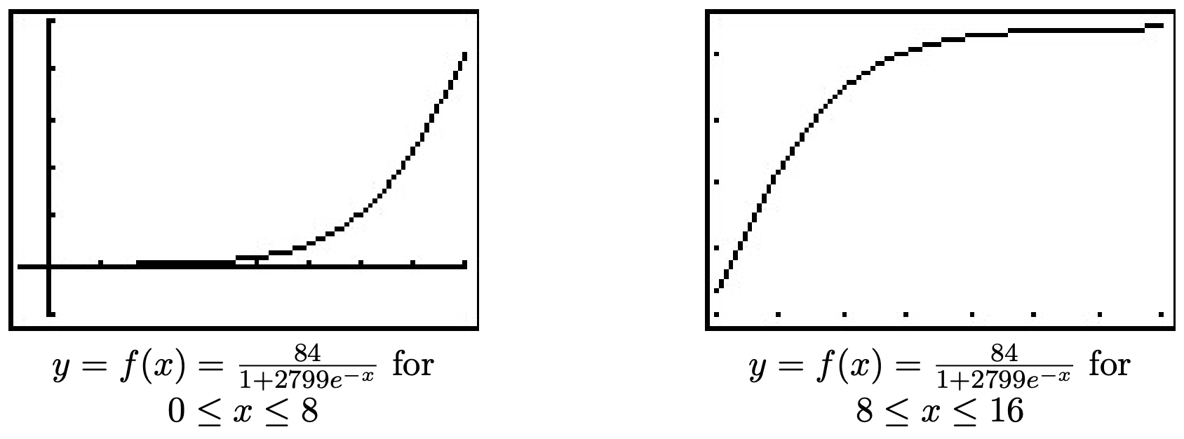
The number of people \(P\), in hundreds, at a local community college who have heard the rumor "Carl is afraid of Virginia Woolf" can be modeled using the logistic equation \[P(t) = \frac{84}{1+2799e^{-t}},\nonumber\]where \(t\geq 0\) is the number of days after April 1, 2009.

1. Find and interpret \(P(0)\).
2. Find and interpret the end behavior of \(P(t)\).
3. How long until \(4200\) people have heard the rumor?
4. Check your answers to 2 and 3 using your calculator.

Solution

1. We find \(P(0) = \frac{84}{1+2799e^{0}} = \dfrac{84}{2800} = \dfrac{3}{100}\). Since \(P(t)\) measures the number of people who have heard the rumor in hundreds, \(P(0)\) corresponds to \(3\) people. Since \(t=0\) corresponds to April 1, 2009, we may conclude that on that day, \(3\) people have heard the rumor.
2. We could simply note that \(P(t)\) is written in the form of the logistic growth model, and identify \(L = 84\). However, to see why the answer is \(84\), we proceed analytically. Since the domain of \(P\) is restricted to \(t \geq 0\), the only end behavior of significance is \(t \to \infty\). As we’ve seen before,¹⁵ as \(t \to \infty\), we have \(1997 e^{-t} \to 0^{+}\) and so \(P(t) \approx \frac{84}{1+\text { very small }(+)} \approx 84\). Hence, as \(t \to \infty\), \(P(t) \to 84\). This means that as time goes by, the number of people who will have heard the rumor approaches \(8400\).
3. To find how long it takes until \(4200\) people have heard the rumor, we set \(P(t) = 42\). Solving \(\frac{84}{1+2799e^{-t}} = 42\) gives \(t = \ln(2799) \approx 7.937\). It takes around \(8\) days until \(4200\) people have heard the rumor.
4. We graph \(y=P(x)\) using the calculator and see that the line \(y=84\) is the horizontal asymptote of the graph, confirming our answer to part 2, and the graph intersects the line \(y=42\) at \(x = \ln(2799) \approx 7.937\), which confirms our answer to part 3.

   

If we take the time to analyze the graph of \(y=P(x)\) above, we can see graphically how logistic growth combines features of uninhibited and limited growth. The curve seems to rise steeply, then at some point, begins to level off. The point at which this happens is called an inflection point or is sometimes called the "point of diminishing returns." At this point, even though the function is still increasing, the rate at which it does so begins to decline. It turns out the point of diminishing returns always occurs at half the limiting population. (In our case, when \(y=42\).) While these concepts are more precisely quantified using Calculus, below are two views of the graph of \(y=P(x)\), one on the interval \([0,8]\), the other on \([8,15]\). The former looks strikingly like uninhibited growth; the latter like limited growth.

Subsection Footnotes

¹³ At which point it would be more toast than roast.

¹⁴ That is, as \(t \to \infty, P(t) \to L\).

¹⁵ See, for example, Example 6.1.2.

---

Applications of Logarithmic Functions

Just as many physical phenomena can be modeled by exponential functions, the same is true of logarithmic functions. In a few of the homework exercises in Section 6.1, we showed that logarithms are useful in measuring the intensities of earthquakes (the Richter scale), sound (decibels) and acids and bases (pH). We now present yet a different use of the a basic logarithm function, password strength.

Example \( \PageIndex{6} \)

The information entropy \(H\), in bits, of a randomly generated password consisting of \(L\) characters is given by \[H = L \log_{2}(N),\nonumber\]where \(N\) is the number of possible symbols for each character in the password. In general, the higher the entropy, the stronger the password.

1. If a \(7\) character case-sensitive¹⁶ password is comprised of letters and numbers only, find the associated information entropy.
2. How many possible symbol options per character is required to produce a \(7\) character password with an information entropy of \(50\) bits?

Solution

1. There are \(26\) letters in the alphabet, \(52\) if upper and lower case letters are counted as different. There are \(10\) digits (\(0\) through \(9\)) for a total of \(N=62\) symbols. Since the password is to be \(7\) characters long, \(L = 7\). Thus, \(H = 7 \log_{2}(62) = \frac{7 \ln(62)}{\ln(2)} \approx 41.68\).
2. We have \(L = 7\) and \(H=50\) and we need to find \(N\). Solving the equation \(50 = 7 \log_{2}(N)\) gives \(N = 2^{50/7} \approx 141.323\), so we would need \(142\) different symbols to choose from.¹⁷

Chemical systems known as buffer solutions have the ability to adjust to small changes in acidity to maintain a range of pH values. Buffer solutions have a wide variety of applications from maintaining a healthy fish tank to regulating the pH levels in blood. Our next example shows how the pH in a buffer solution is a little more complicated than the pH we first encountered in the homework exercises of Section 6.1.

Example \( \PageIndex{7} \)

Blood is a buffer solution. When carbon dioxide is absorbed into the bloodstream it produces carbonic acid and lowers the pH. The body compensates by producing bicarbonate, a weak base to partially neutralize the acid. The equation¹⁸ which models blood pH in this situation is \[\text{pH} = 6.1 + \log\left(\frac{800}{x} \right),\nonumber\]where \(x\) is the partial pressure of carbon dioxide in arterial blood, measured in torr. Find the partial pressure of carbon dioxide in arterial blood if the pH is \(7.4\).

Solution

We set \(\mbox{pH} = 7.4\) and get \(7.4 = 6.1 + \log\left(\frac{800}{x} \right)\), or \(\log\left(\frac{800}{x} \right) = 1.3\). Solving, we find \(x = \frac{800}{10^{1.3}} \approx 40.09\). Hence, the partial pressure of carbon dioxide in the blood is about \(40\) torr.

Subsection Footnotes

¹⁶ That is, upper and lower case letters are treated as different characters.

¹⁷ Since there are only 94 distinct ASCII keyboard characters, to achieve this strength, the number of characters in the password should be increase.

¹⁸ Derived from the Henderson-Hasselbalch Equation (see the homework in Section 6.2). Hasselbalch himself was studying carbon dioxide dissolving in blood - a process called metabolic acidosis.